FictionArt - Data Cleaning

Data Preparation

library(tidyverse)
library(easystats)
library(patchwork)
library(ggside)
library(ggdist)
library(brms)


df <- read.csv("../data/data_memory_task.csv") |> 
  mutate(Condition = fct_relevel(Condition, "Human Original", "Human Forgery", "AI-Generated", "New Items"),
         AnswerCondition = fct_relevel(AnswerCondition, "Human Original", "Human Forgery", "AI-Generated", "Not recognized"),
         AnswerBelief = fct_relevel(AnswerBelief, "Human Original", "Human Forgery", "AI Original", "AI Copy", "Not recognized"),
         Belief = fct_relevel(Belief, "Human Original", "Human Forgery", "AI Original", "AI Copy", "None"))

dfsub <- read.csv("../data/data_participants.csv") |> 
  filter(Participant %in% df$Participant)

cols <- c(
  # Condition
  "Human Original" = "#F51D56",
  "Human Forgery" = "#F5A41D",
  "AI-Generated" = "#1D9AF5",
  "AI Original" = "#1D9AF5",
  "AI Copy" = "#4CAF50",
  "Not recognized" = "#607D8B",
  # Style
  "Abstract and Avant-garde" = "#E41A1C", 
  "Classical" = "#377EB8", 
  "Impressionist and Expressionist" = "#4DAF4A", 
  "Romantic and Realism" = "#FF7F00"
)

Delay

Code

dfsub |> 
  ggplot(aes(x=Delay)) +
  geom_histogram(bins=30) +
  theme_minimal()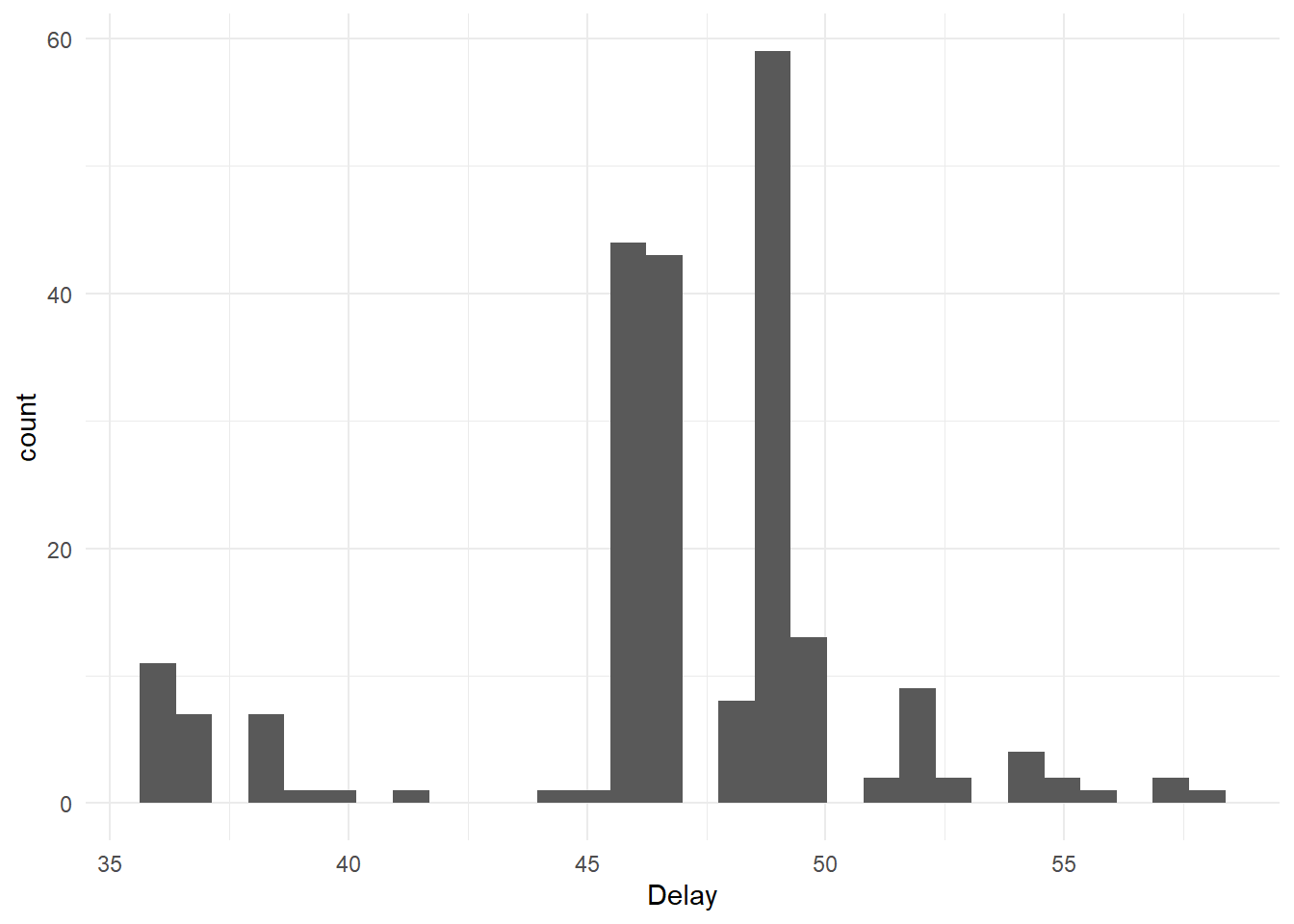

The mean and median days between the two experiments were 46.95 and 47.00, respectively.

Memory of Condition

Main

Code

m_cond1 <- brm(AnswerCondition ~ Condition + (1|Participant) + (1|Item),
    data = df,
    family = categorical(link = "logit"),
    algorithm = "meanfield",
    iter = 8000,
    backend = "cmdstanr")

------------------------------------------------------------ 
EXPERIMENTAL ALGORITHM: 
  This procedure has not been thoroughly tested and may be unstable 
  or buggy. The interface is subject to change. 
------------------------------------------------------------ 
Gradient evaluation took 0.061406 seconds 
1000 transitions using 10 leapfrog steps per transition would take 614.06 seconds. 
Adjust your expectations accordingly! 
Begin eta adaptation. 
Iteration:   1 / 250 [  0%]  (Adaptation) 
Iteration:  50 / 250 [ 20%]  (Adaptation) 
Iteration: 100 / 250 [ 40%]  (Adaptation) 
Iteration: 150 / 250 [ 60%]  (Adaptation) 
Iteration: 200 / 250 [ 80%]  (Adaptation) 
Success! Found best value [eta = 1] earlier than expected. 
Begin stochastic gradient ascent. 
  iter             ELBO   delta_ELBO_mean   delta_ELBO_med   notes  
   100       -15455.677             1.000            1.000 
   200       -14802.122             0.522            1.000 
   300       -14672.904             0.351            0.044 
   400       -14650.076             0.264            0.044 
   500       -14647.462             0.211            0.009   MEDIAN ELBO CONVERGED 
Drawing a sample of size 1000 from the approximate posterior...  
COMPLETED. 
Finished in  23.8 seconds.

Code

# Modify the order of dodging based on the groups for visualization
make_group <- function(resp, covariate = NULL) {
  group <- case_when(  
    resp == "Not recognized" ~ 0,
    resp == "Human Original" ~ 1,
    resp == "AI-Generated" ~ 2,
    resp == "AI Original" ~ 2,
    resp == "Human Forgery" ~ 3,
    resp == "AI Copy" ~ 4,
    .default = NA)
  
  if(!is.null(covariate)) {
    covariate <- insight::format_value(normalize(covariate), style_positive="plus")
    group <- paste0(group, covariate)
  }
  group
}

dat_cond1 <- estimate_means(m_cond1, by=c("Condition")) |> 
  mutate(group = make_group(Response))

p_cond1 <- dat_cond1 |> 
  ggplot(aes(x=Condition,  y = Median, color = Response)) +
  geom_line(aes(group=group), position = position_dodge(width=0.1), linewidth = 1,
            show.legend = FALSE) +
  geom_pointrange(aes(group=group, ymin = CI_low, ymax = CI_high), position = position_dodge(width=0.1),
                  key_glyph = "point") +
  scale_y_continuous(label = scales::percent, limits = c(0,1), expand = c(0, 0)) +
  scale_color_manual(values = cols) +
  guides(color = guide_legend(override.aes = list(size = 3))) +
  labs(y="Proportion of answers", color = "Answer", x =  "Experimental Condition",
       title = "Memory of the Experimental Condition") +
  theme_minimal() 
p_cond1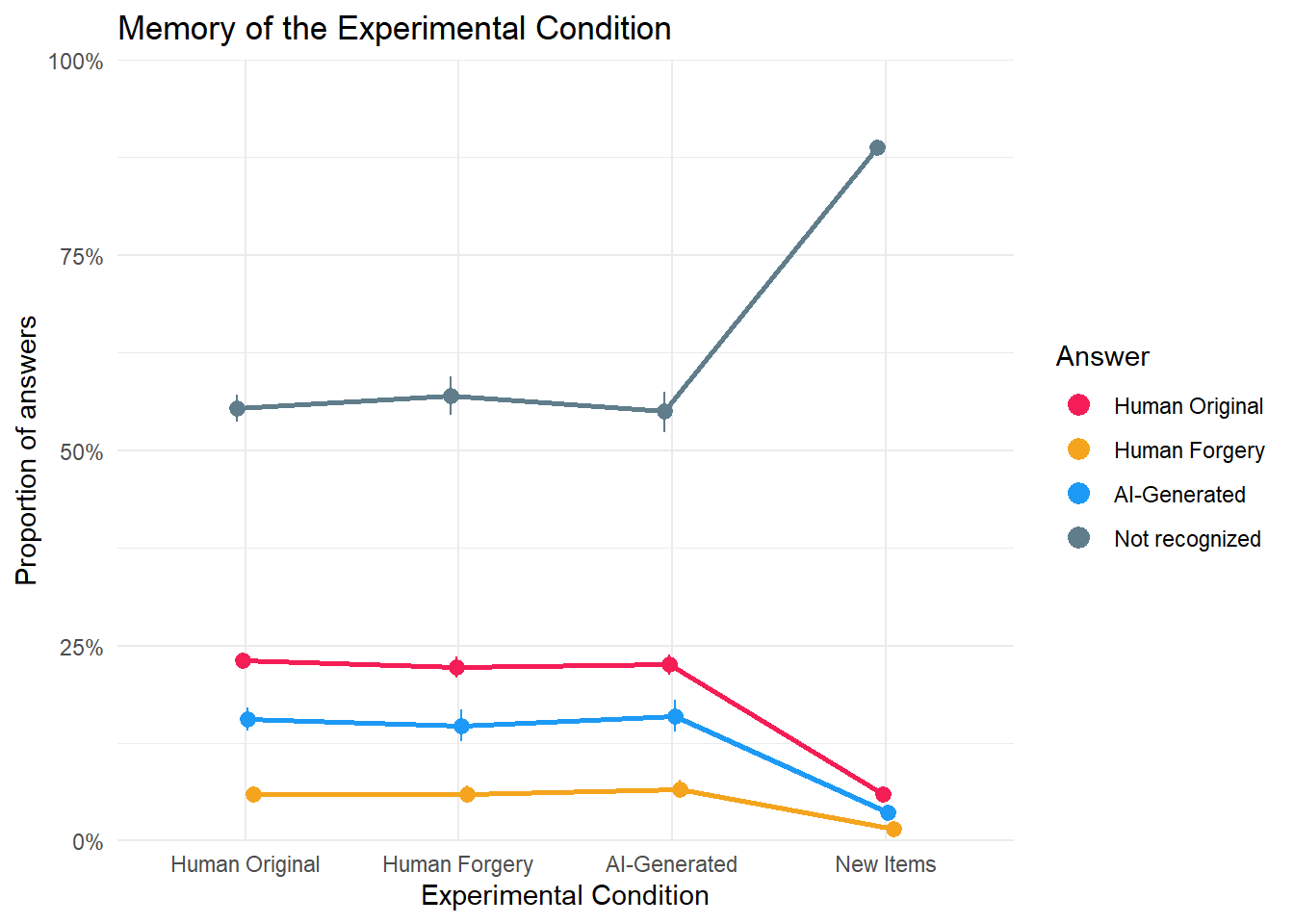

Code

make_contrasts <- function(c, answer=NULL, condition=NULL) {
  # We can detect via the space because answer comes first
  c$Response1 <- case_when(
    str_detect(c$Level1, "Human Original ") ~ "Human Original",
    str_detect(c$Level1, "Human Forgery ") ~ "Human Forgery",
    str_detect(c$Level1, "AI-Generated ") ~ "AI-Generated",
    str_detect(c$Level1, "Not recognized ") ~ "Not recognized",
    str_detect(c$Level1, "AI Copy ") ~ "AI Copy",
    str_detect(c$Level1, "AI Original ") ~ "AI Original",
    .default = NA
  )
  c$Response2 <- case_when(
    str_detect(c$Level2, "Human Original ") ~ "Human Original",
    str_detect(c$Level2, "Human Forgery ") ~ "Human Forgery",
    str_detect(c$Level2, "AI-Generated ") ~ "AI-Generated",
    str_detect(c$Level2, "Not recognized ") ~ "Not recognized",
    str_detect(c$Level2, "AI Copy ") ~ "AI Copy",
    str_detect(c$Level2, "AI Original ") ~ "AI Original",
    .default = NA
  )
  c$Level1 <- str_remove(c$Level1, "Human Original |Human Forgery |AI-Generated |Not recognized |AI Original |AI Copy ")
  c$Level2 <- str_remove(c$Level2, "Human Original |Human Forgery |AI-Generated |Not recognized |AI Original |AI Copy ")
  
  if(!is.null(answer)) {
    c <- filter(c, str_detect(Response1, answer) & str_detect(Response2, answer))
  }
  if(!is.null(condition)) {
    c <- filter(c, str_detect(Level1, condition) & str_detect(Level2, condition))
  }
  
  # Remove duplicated cols
  if(length(unique(c$Response1)) == 1 & all(c$Response1 == c$Response2)) {
    c <- cbind(data.frame("Category" = c$Response1[1]), c)
    c$Response1 <- NULL
    c$Response2 <- NULL
  }
  if(length(unique(c$Level1)) == 1 & all(c$Level1 == c$Level2)) {
    c <- cbind(data.frame("Category" = c$Level1[1]), c)
    c$Level1 <- NULL
    c$Level2 <- NULL
  }
  
  c <- arrange(c, desc(abs(Median))) 
  t <- format_table(c, zap_small = TRUE)
  
  t$effectsize <- as.numeric(c$Median)
  t$sig <- as.numeric(c$pd)
  
  gt::gt(t) |> 
    gt::data_color(columns = "effectsize", target_columns = "Median", method = "numeric",
palette = c("red", "red", "white", "green", "green"), domain = c(-0.7, 0.7)) |> 
    gt::data_color(columns = "sig", target_columns = "pd", fn = \(x) {
      ifelse(x > 0.99, "#FFC107", ifelse(x > 0.97, "#FFEB3B", ifelse(x > 0.95, "#FFF59D", "white")))
    }) |> 
    gt::cols_hide(c("effectsize", "sig")) |> 
    gt::tab_header(title = "Marginal Contrasts")
}

c <- estimate_contrasts(m_cond1, contrast = c("Condition"), test = "pd")
make_contrasts(c, answer="Not recognized")

Category	Level1	Level2	Median	CI	pd
Marginal Contrasts
Not recognized	New Items	AI-Generated	0.34	[ 0.31, 0.36]	100%
Not recognized	New Items	Human Original	0.33	[ 0.32, 0.35]	100%
Not recognized	New Items	Human Forgery	0.32	[ 0.29, 0.34]	100%
Not recognized	AI-Generated	Human Forgery	-0.02	[-0.05, 0.01]	90.50%
Not recognized	Human Forgery	Human Original	0.02	[-0.01, 0.04]	92.20%
Not recognized	AI-Generated	Human Original	0.00	[-0.03, 0.02]	65.20%

Code

make_contrasts(c, condition="Human Original")

Category	Median	CI	pd	Response1	Response2
Marginal Contrasts
Human Original	0.49	[ 0.47, 0.51]	100%	Not recognized	Human Forgery
Human Original	0.40	[ 0.37, 0.43]	100%	Not recognized	AI-Generated
Human Original	0.32	[ 0.30, 0.35]	100%	Not recognized	Human Original
Human Original	-0.17	[-0.18, -0.16]	100%	Human Forgery	Human Original
Human Original	0.10	[ 0.08, 0.11]	100%	AI-Generated	Human Forgery
Human Original	-0.08	[-0.09, -0.06]	100%	AI-Generated	Human Original

Code

make_contrasts(c, condition="New Items")

Warning: Some values were outside the color scale and will be treated as NA

Category	Median	CI	pd	Response1	Response2
Marginal Contrasts
New Items	0.87	[ 0.86, 0.88]	100%	Not recognized	Human Forgery
New Items	0.85	[ 0.84, 0.86]	100%	Not recognized	AI-Generated
New Items	0.83	[ 0.82, 0.84]	100%	Not recognized	Human Original
New Items	-0.04	[-0.05, -0.04]	100%	Human Forgery	Human Original
New Items	-0.02	[-0.03, -0.02]	100%	AI-Generated	Human Original
New Items	0.02	[ 0.02, 0.03]	100%	AI-Generated	Human Forgery

Self-Relevance

Code

m_cond2a <- brm(AnswerCondition ~ Condition * SelfRelevance + (1|Participant),
    data = df,
    family = categorical(link = "logit"),
    algorithm = "meanfield",
    iter = 8000,
    backend = "cmdstanr")

Warning: Rows containing NAs were excluded from the model.

------------------------------------------------------------ 
EXPERIMENTAL ALGORITHM: 
  This procedure has not been thoroughly tested and may be unstable 
  or buggy. The interface is subject to change. 
------------------------------------------------------------ 
Gradient evaluation took 0.010415 seconds 
1000 transitions using 10 leapfrog steps per transition would take 104.15 seconds. 
Adjust your expectations accordingly! 
Begin eta adaptation. 
Iteration:   1 / 250 [  0%]  (Adaptation) 
Iteration:  50 / 250 [ 20%]  (Adaptation) 
Iteration: 100 / 250 [ 40%]  (Adaptation) 
Iteration: 150 / 250 [ 60%]  (Adaptation) 
Iteration: 200 / 250 [ 80%]  (Adaptation) 
Success! Found best value [eta = 1] earlier than expected. 
Begin stochastic gradient ascent. 
  iter             ELBO   delta_ELBO_mean   delta_ELBO_med   notes  
   100       -10981.965             1.000            1.000 
   200       -10899.023             0.504            1.000 
   300       -10886.602             0.336            0.008   MEDIAN ELBO CONVERGED 
Drawing a sample of size 1000 from the approximate posterior...  
COMPLETED. 
Finished in  11.1 seconds.

Code

dat_cond2a <- estimate_means(m_cond2a, by=c("Condition", "SelfRelevance"), length = 7) |> 
  mutate(group = make_group(Response, SelfRelevance),
         SelfRelevance = fct_reorder(format_percent(SelfRelevance, digits = 0), SelfRelevance))

p_cond2a <- dat_cond2a |> 
  ggplot(aes(x=Condition,  y = Median, color = Response)) +
  geom_line(aes(group=group, alpha=SelfRelevance), position = position_dodge(width=0.2), linewidth = 1,
            show.legend = c(color = FALSE)) +
  geom_pointrange(aes(group=group, ymin = CI_low, ymax = CI_high, alpha=SelfRelevance), position = position_dodge(width=0.2),
                  show.legend = c(alpha = FALSE), key_glyph = "point") +
  scale_y_continuous(label = scales::percent, limits = c(0,1), expand = c(0, 0)) +
  scale_color_manual(values = cols) +
  scale_alpha_discrete(breaks = c("0%", "50%", "100%")) +
  guides(color = guide_legend(override.aes = list(size = 3))) +
  labs(y="Proportion of answers", color = "Answer", x =  "Experimental Condition",
       title = "Effect of Self-Relevance") +
  theme_minimal()

Warning: Using alpha for a discrete variable is not advised.

Code

p_cond2a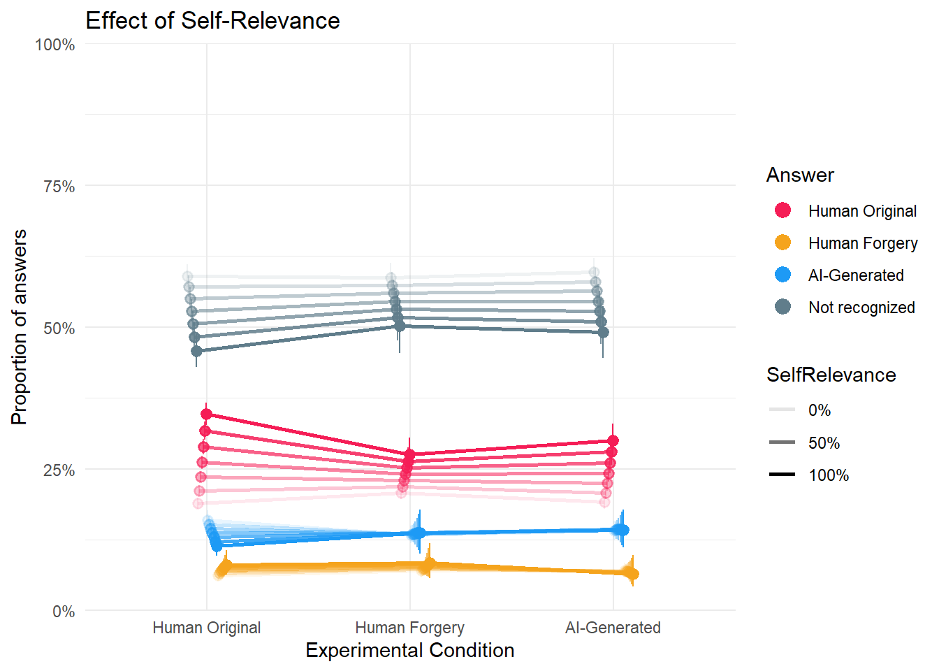

Code

c <- estimate_contrasts(m_cond2a, contrast = c("Condition", "SelfRelevance"), test = "pd")

# Specific contrast
c[c$Parameter == "Human Original Human Original 1.000 - Human Original Human Original 0.000",]

Marginal Contrasts Analysis

Parameter                                                                
-------------------------------------------------------------------------
Human Original Human Original 1.000 - Human Original Human Original 0.000

Median |       95% CI |   pd
----------------------------
  0.16 | [0.14, 0.18] | 100%

Variable predicted: AnswerCondition
Predictors contrasted: Condition, SelfRelevance
Predictors averaged: Participant
Contrasts are on the response-scale.

Beauty

Code

m_cond2b <- brm(AnswerCondition ~ Condition * poly(Beauty, 2) + (1|Participant),
    data = filter(df, !is.na(Beauty)),
    family = categorical(link = "logit"),
    algorithm = "meanfield",
    iter = 8000,
    backend = "cmdstanr")

------------------------------------------------------------ 
EXPERIMENTAL ALGORITHM: 
  This procedure has not been thoroughly tested and may be unstable 
  or buggy. The interface is subject to change. 
------------------------------------------------------------ 
Gradient evaluation took 0.009251 seconds 
1000 transitions using 10 leapfrog steps per transition would take 92.51 seconds. 
Adjust your expectations accordingly! 
Begin eta adaptation. 
Iteration:   1 / 250 [  0%]  (Adaptation) 
Iteration:  50 / 250 [ 20%]  (Adaptation) 
Iteration: 100 / 250 [ 40%]  (Adaptation) 
Iteration: 150 / 250 [ 60%]  (Adaptation) 
Iteration: 200 / 250 [ 80%]  (Adaptation) 
Success! Found best value [eta = 1] earlier than expected. 
Begin stochastic gradient ascent. 
  iter             ELBO   delta_ELBO_mean   delta_ELBO_med   notes  
   100       -11736.702             1.000            1.000 
   200       -11000.482             0.533            1.000 
   300       -10967.195             0.357            0.067 
   400       -10860.314             0.270            0.067 
   500       -10843.136             0.216            0.010   MEDIAN ELBO CONVERGED 
Drawing a sample of size 1000 from the approximate posterior...  
COMPLETED. 
Finished in  13.3 seconds.

Code

dat_cond2b <- estimate_means(m_cond2b, by=c("Condition", "Beauty"), length = 7) |> 
  mutate(group = make_group(Response, Beauty),
         Beauty = fct_reorder(format_percent(Beauty, digits = 0), Beauty))

p_cond2b <- dat_cond2b |> 
  ggplot(aes(x=Condition,  y = Median, color = Response)) +
  # geom_line(aes(group=group, alpha=Beauty), position = position_dodge(width=0.8), linewidth = 1) +
  geom_pointrange(aes(ymin = CI_low, ymax = CI_high, alpha=Beauty), position = position_dodge(width=0.8),
                  show.legend = c(alpha = FALSE), key_glyph = "point") +
  scale_y_continuous(label = scales::percent, limits = c(0,1), expand = c(0, 0)) +
  scale_color_manual(values = cols) +
  scale_alpha_discrete(breaks = c("0%", "50%", "100%")) +
  guides(alpha = "none", color = guide_legend(override.aes = list(size = 3))) +
  labs(y="Proportion of answers", color = "Answer", x =  "Experimental Condition",
       title = "Effect of Beauty") +
  theme_minimal()

Warning: Using alpha for a discrete variable is not advised.

Code

p_cond2b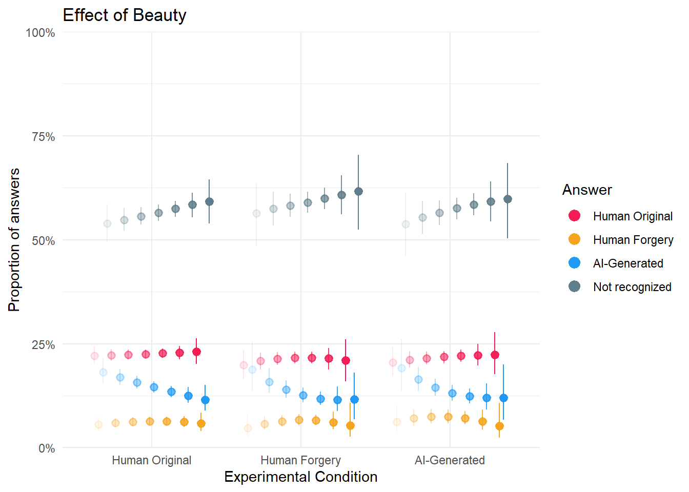

Code

((p_cond1 + theme(legend.position = "none")) | (p_cond2a / p_cond2b) +
  plot_layout(guides = "collect")) + 
  plot_annotation(title = "Do you remember how this artwork was labelled?", theme = theme(plot.title = element_text(hjust = 0.5, face="italic", size=rel(1.5))))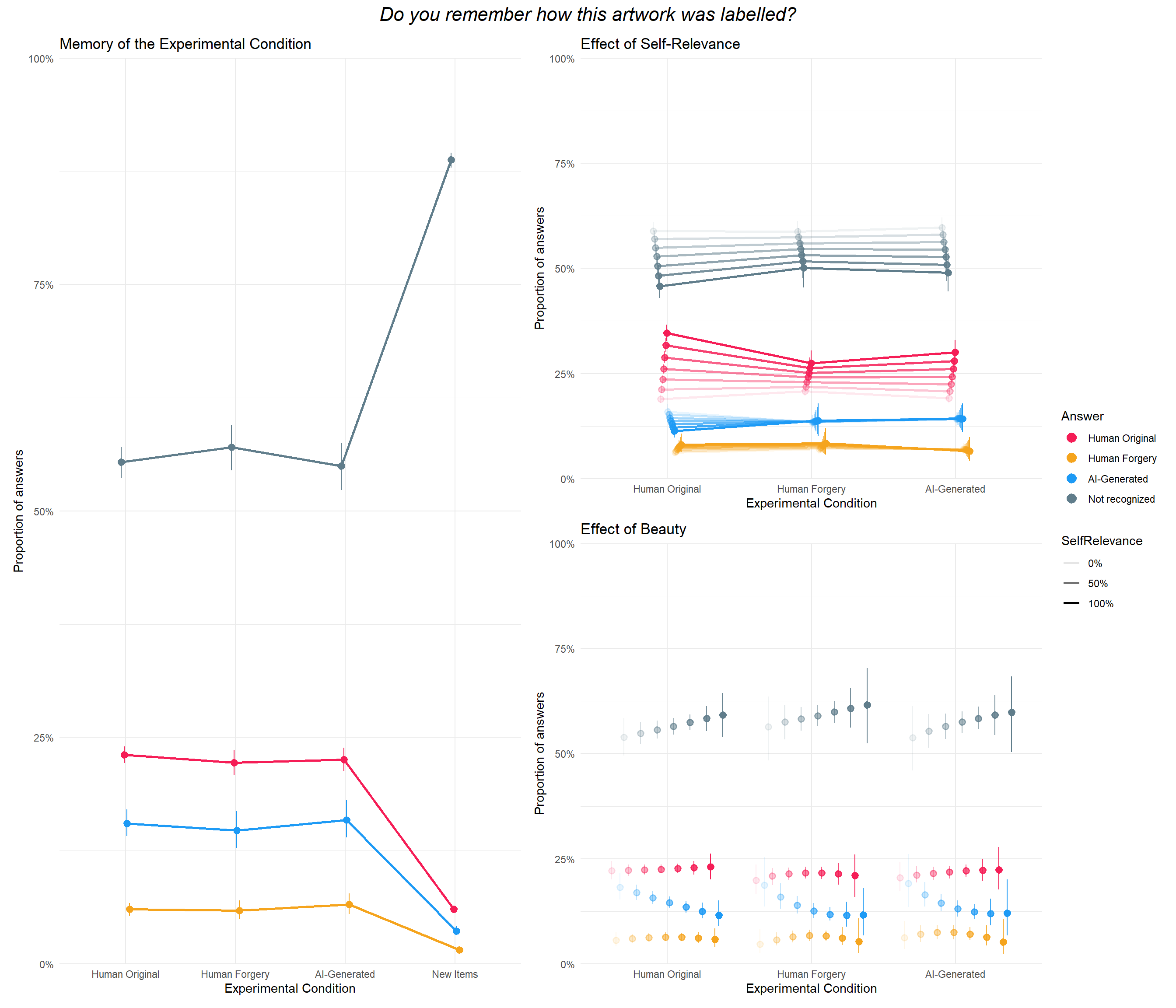

Memory of Beliefs

Main

Code

m_belief1a <- brm(AnswerBelief ~ Belief + (1|Participant),
    data = df,
    family = categorical(link = "logit"),
    algorithm = "meanfield",
    iter = 8000,
    backend = "cmdstanr")

------------------------------------------------------------ 
EXPERIMENTAL ALGORITHM: 
  This procedure has not been thoroughly tested and may be unstable 
  or buggy. The interface is subject to change. 
------------------------------------------------------------ 
Gradient evaluation took 0.020273 seconds 
1000 transitions using 10 leapfrog steps per transition would take 202.73 seconds. 
Adjust your expectations accordingly! 
Begin eta adaptation. 
Iteration:   1 / 250 [  0%]  (Adaptation) 
Iteration:  50 / 250 [ 20%]  (Adaptation) 
Iteration: 100 / 250 [ 40%]  (Adaptation) 
Iteration: 150 / 250 [ 60%]  (Adaptation) 
Iteration: 200 / 250 [ 80%]  (Adaptation) 
Success! Found best value [eta = 1] earlier than expected. 
Begin stochastic gradient ascent. 
  iter             ELBO   delta_ELBO_mean   delta_ELBO_med   notes  
   100       -16788.145             1.000            1.000 
   200       -16645.913             0.504            1.000 
   300       -16645.766             0.336            0.009   MEDIAN ELBO CONVERGED 
Drawing a sample of size 1000 from the approximate posterior...  
COMPLETED. 
Finished in  19.0 seconds.

Code

dat_belief1a <- estimate_means(m_belief1a, by=c("Belief")) |> 
  mutate(group = make_group(Response))

p_belief1a <- dat_belief1a |> 
  ggplot(aes(x=Belief,  y = Median, color = Response)) +
  geom_line(aes(group=group), position = position_dodge(width=0.1), linewidth = 1, 
            show.legend = FALSE) +
  geom_pointrange(aes(group=group, ymin = CI_low, ymax = CI_high), position = position_dodge(width=0.1),
                  key_glyph = "point") +
  scale_y_continuous(label = scales::percent, limits = c(0,1), expand = c(0, 0)) +
  scale_color_manual(values = cols) +
  guides(color = guide_legend(override.aes = list(size = 3))) +
  labs(y="Proportion of answers", color = "Answer", x =  "Original Belief",
       title = "Memory of Beliefs") +
  theme_minimal()
p_belief1a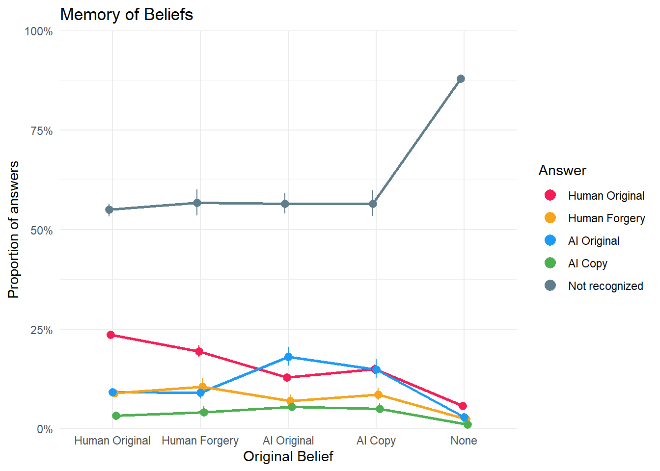

Code

c <- estimate_contrasts(m_belief1a, contrast = c("Belief"), test = "pd")
make_contrasts(c, answer="Not recognized")

Category	Level1	Level2	Median	CI	pd
Marginal Contrasts
Not recognized	None	Human Original	0.33	[ 0.31, 0.35]	100%
Not recognized	None	AI Original	0.31	[ 0.29, 0.34]	100%
Not recognized	None	AI Copy	0.31	[ 0.28, 0.35]	100%
Not recognized	None	Human Forgery	0.31	[ 0.28, 0.34]	100%
Not recognized	Human Forgery	Human Original	0.02	[-0.02, 0.05]	88.50%
Not recognized	AI Copy	Human Original	0.02	[-0.02, 0.05]	82.50%
Not recognized	AI Original	Human Original	0.02	[-0.01, 0.04]	91.80%
Not recognized	AI Original	Human Forgery	0.00	[-0.04, 0.04]	52.90%
Not recognized	AI Copy	Human Forgery	0.00	[-0.05, 0.04]	51.90%
Not recognized	AI Copy	AI Original	0.00	[-0.04, 0.04]	51.70%

Code

make_contrasts(c, condition="Human Original")

Category	Median	CI	pd	Response1	Response2
Marginal Contrasts
Human Original	0.52	[ 0.50, 0.53]	100%	Not recognized	AI Copy
Human Original	0.46	[ 0.44, 0.48]	100%	Not recognized	Human Forgery
Human Original	0.46	[ 0.44, 0.48]	100%	Not recognized	AI Original
Human Original	0.31	[ 0.29, 0.33]	100%	Not recognized	Human Original
Human Original	-0.20	[-0.21, -0.19]	100%	AI Copy	Human Original
Human Original	-0.15	[-0.16, -0.13]	100%	Human Forgery	Human Original
Human Original	-0.14	[-0.16, -0.13]	100%	AI Original	Human Original
Human Original	-0.06	[-0.07, -0.05]	100%	AI Copy	AI Original
Human Original	-0.06	[-0.07, -0.04]	100%	AI Copy	Human Forgery
Human Original	0.00	[-0.01, 0.02]	66.20%	AI Original	Human Forgery

Continuous

Code

m_belief1b <- brm(AnswerBelief ~ poly(Reality, 2) * poly(Authenticity, 2) + (1|Participant),
    data = filter(df, Type == "Old", !is.na(Reality)),
    family = categorical(link = "logit"),
    algorithm = "meanfield",
    iter = 12000,
    backend = "cmdstanr")

------------------------------------------------------------ 
EXPERIMENTAL ALGORITHM: 
  This procedure has not been thoroughly tested and may be unstable 
  or buggy. The interface is subject to change. 
------------------------------------------------------------ 
Gradient evaluation took 0.009641 seconds 
1000 transitions using 10 leapfrog steps per transition would take 96.41 seconds. 
Adjust your expectations accordingly! 
Begin eta adaptation. 
Iteration:   1 / 250 [  0%]  (Adaptation) 
Iteration:  50 / 250 [ 20%]  (Adaptation) 
Iteration: 100 / 250 [ 40%]  (Adaptation) 
Iteration: 150 / 250 [ 60%]  (Adaptation) 
Iteration: 200 / 250 [ 80%]  (Adaptation) 
Success! Found best value [eta = 1] earlier than expected. 
Begin stochastic gradient ascent. 
  iter             ELBO   delta_ELBO_mean   delta_ELBO_med   notes  
   100       -11794.023             1.000            1.000 
   200       -11704.251             0.504            1.000 
   300       -11642.760             0.338            0.008   MEDIAN ELBO CONVERGED 
Drawing a sample of size 1000 from the approximate posterior...  
COMPLETED. 
Finished in  13.5 seconds.

Code

dat_belief1b <- estimate_means(m_belief1b, by=c("Reality", "Authenticity"), length = c(13, 5)) |> 
  mutate(
    group = make_group(Response, Authenticity),
    Authenticity = fct_reorder(format_percent(Authenticity, digits = 0), Authenticity))

p_belief1b <- dat_belief1b |> 
  ggplot(aes(x=Reality,  y = Median, color = Response)) +
  geom_line(aes(group=group, alpha=Authenticity), position = position_dodge(width=0.2), linewidth = 1,
                  key_glyph = "path", show.legend = c(color = FALSE)) +
  geom_pointrange(data=filter(dat_belief1b, round(Reality, 6) %in% c(0, 0.5, 1)),
                  aes(group=group, ymin = CI_low, ymax = CI_high, alpha=Authenticity), position = position_dodge(width=0.2),
                  key_glyph = "point", show.legend = c(alpha = FALSE)) +
  scale_y_continuous(labels = scales::percent, limits = c(0,0.8), expand = c(0, 0)) +
  scale_x_continuous(labels = scales::percent, breaks = c(0, 0.5, 1)) +
  scale_color_manual(values = cols) +
  scale_alpha_discrete(breaks = c("0%", "50%", "100%")) +
  guides(color = "none") +
  labs(y="Proportion of answers", color = "Answer", x =  "AI vs. Human", alpha  = "Copy vs. Original",
       title = "Continuous Effect of Beliefs") +
  theme_minimal() +
  facet_grid(~Response)

Warning: Using alpha for a discrete variable is not advised.

Code

p_belief1b

Warning: `position_dodge()` requires non-overlapping x intervals.

Warning: `position_dodge()` requires non-overlapping x intervals.
`position_dodge()` requires non-overlapping x intervals.
`position_dodge()` requires non-overlapping x intervals.
`position_dodge()` requires non-overlapping x intervals.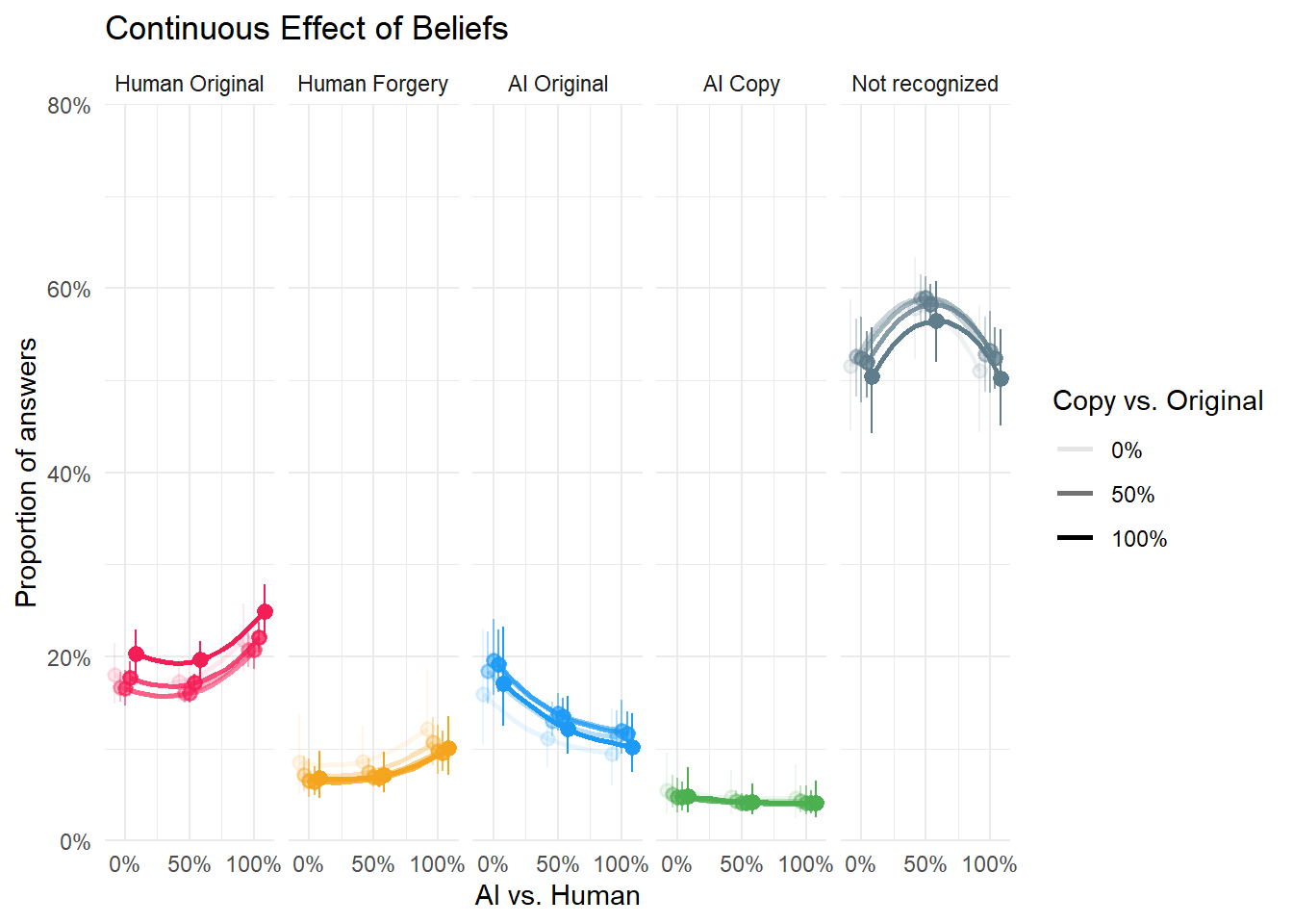

Code

p_belief1a / p_belief1b + 
  plot_layout(guides = "collect") + 
  plot_annotation(title = "Do you remember your own judgments?",
                  theme = theme(plot.title = element_text(hjust = 0.5, face="italic", size=rel(1.5))))

Warning: `position_dodge()` requires non-overlapping x intervals.
`position_dodge()` requires non-overlapping x intervals.
`position_dodge()` requires non-overlapping x intervals.
`position_dodge()` requires non-overlapping x intervals.
`position_dodge()` requires non-overlapping x intervals.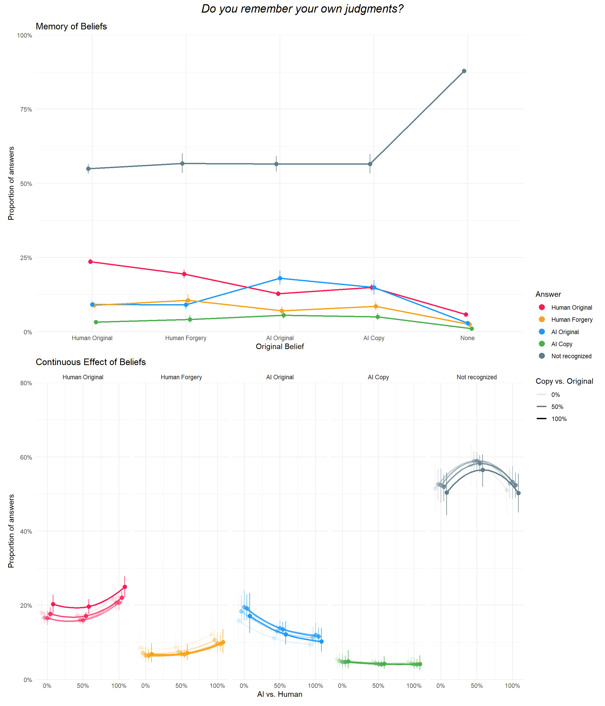

Participant-level

In this recognition task, in which people were presented old and new items, and had to 1) answer if they recognize it or not, and if so then remember the condition it was presented in as well as the memory of their own belief that they had about the item.

Compute Indidces

dprime: Sensitivity index quantifying how well a participant discriminates old from new items. Higher values indicate better recognition accuracy; 0 reflects chance-level discrimination.
c : Parametric response bias criterion. Negative values indicate a liberal bias (more “old” responses), positive values a conservative bias (more “new” responses), and 0 indicates no bias.
BiasCondition_Human: Among all recognised items, the proportion labelled Human Original. Higher values indicate a stronger tendency to classify recognised items as human, regardless of their original condition assignment.
BiasCondition_Forgery: Among all recognised items, the proportion labelled Human Forgery. This reflects a bias towards attributing recognised items to manipulated human sources, regardless of their original condition assignment.
BiasCondition_AI: Among all recognised items, the proportion labelled AI-Generated. Higher values indicate a stronger general tendency to attribute recognised items to AI, regardless of their original condition assignment.
BiasBelief_HumanOriginal: Proportion of recognised items for which participants remember having believed they were Human Original.
BiasBelief_HumanForgery: Proportion remembered as Human Forgery, indicating recalled suspicion of human tampering.
BiasBelief_AIOriginal: Proportion remembered as AI Original, indicating remembered beliefs that items were originally produced by AI.
BiasBelief_AICopy: Proportion remembered as AI Copy, reflecting recalled beliefs that items were AI-generated and derivative.
BiasBelief_Human: Combined proportion of Human Original + Human Forgery. Represents the tendency to remember having believed items were human rather than AI.
BiasBelief_Authentic: Combined proportion of Human Original + AI Original. Captures the tendency to recall having believed items were “authentic” originals rather than copies or forgeries.

Code

# log-linear corrected rates to avoid 0/1 extremes
ll_rate <- function(count, total) {
  (count + 0.5) / (total + 1)
}

# parametric SDT: d' and c
sdt_metrics <- function(hit_rate, fa_rate) {
  # qnorm works with rates strictly in (0,1)
  z_hit <- qnorm(hit_rate)
  z_fa  <- qnorm(fa_rate)
  dprime <- z_hit - z_fa
  criterion_c <- -0.5 * (z_hit + z_fa)
  tibble(dprime = dprime, c = criterion_c)
}

dffeatures <- df |>
  summarise(
    n_old  = sum(Type == "Old", na.rm = TRUE),
    n_new  = sum(Type == "New", na.rm = TRUE),
    hits   = sum(Recognition == "Yes" & Type == "Old", na.rm = TRUE),
    misses = sum(Recognition == "No"  & Type == "Old", na.rm = TRUE),
    fa     = sum(Recognition == "Yes" & Type == "New", na.rm = TRUE),
    cr     = sum(Recognition == "No"  & Type == "New", na.rm = TRUE),
    .by = "Participant"
  ) |>
  mutate(
    p_hit = ll_rate(hits, n_old),
    p_fa  = ll_rate(fa, n_new)
  ) |>
  mutate(
    map2_dfr(p_hit, p_fa, sdt_metrics)
  ) |> 
  select(Participant, dprime, c)

# Condition memory bias
dffeatures <- df |>
  summarise(n = n(), .by = c("Participant", "AnswerCondition")) |> 
  complete(Participant, AnswerCondition, fill = list(n = 0)) |> 
  filter(AnswerCondition != "Not recognized") |> 
  mutate(Total = sum(n), .by = "Participant") |> 
  mutate(p = n / Total) |> 
  select(-n, -Total) |>
  mutate(AnswerCondition = str_replace(AnswerCondition, "AI-Generated", "BiasCondition_AI"),
         AnswerCondition = str_replace(AnswerCondition, "Human Original", "BiasCondition_Human"),
         AnswerCondition = str_replace(AnswerCondition, "Human Forgery", "BiasCondition_Forgery")) |>
  pivot_wider(names_from = AnswerCondition, values_from = p) |> 
  full_join(dffeatures, by = "Participant")

# Belief memory bias
dffeatures <- df |>
  summarise(n = n(), .by = c("Participant", "AnswerBelief")) |> 
  complete(Participant, AnswerBelief, fill = list(n = 0)) |> 
  filter(AnswerBelief != "Not recognized") |> 
  mutate(Total = sum(n), .by = "Participant") |> 
  mutate(p = n / Total) |> 
  select(-n, -Total) |>
  mutate(AnswerBelief = str_replace(AnswerBelief, "AI Original", "BiasBelief_AIOriginal"),
         AnswerBelief = str_replace(AnswerBelief, "AI Copy", "BiasBelief_AICopy"),
         AnswerBelief = str_replace(AnswerBelief, "Human Original", "BiasBelief_HumanOriginal"),
         AnswerBelief = str_replace(AnswerBelief, "Human Forgery", "BiasBelief_HumanForgery")) |>
  pivot_wider(names_from = AnswerBelief, values_from = p) |> 
  mutate(BiasBelief_Human = BiasBelief_HumanOriginal + BiasBelief_HumanForgery,
         BiasBelief_Authentic = BiasBelief_HumanOriginal + BiasBelief_AIOriginal) |>
  full_join(dffeatures, by = "Participant")

Correlation

Code

df2 <- dfsub |> 
  select(Participant, Gender, Age, Education, Delay, Art_Expertise, 
         BAIT_AI_Use, BAIT_AI_Knowledge, BAIT_Negative, BAIT_Positive, BAIT_ArtRealistic, BAIT_Total,
         VVIQ_Total, LifeSatisfaction, PHQ4_Anxiety, PHQ4_Depression, starts_with("MINT_"), -MINT_AttentionCheck) |> 
  mutate(Gender = case_when(
    Gender == "Male" ~ 0,
    Gender == "Female" ~ 1,
    .default =  NA
    ),
    BAIT_AI_Use = case_when(
      BAIT_AI_Use == "Never" ~ 0,
      BAIT_AI_Use == "A few times per month" ~ 1,
      BAIT_AI_Use == "A few times per week" ~ 2,
      BAIT_AI_Use == "Once a day" ~ 3,
      BAIT_AI_Use == "A few times per day" ~ 4,
      .default = NA
    ),
    Education = case_when(
      Education == "High school" ~ 0,
      Education == "Bachelor" ~ 1,
      Education == "Master" ~ 2,
      Education == "Doctorate" ~ 3,
      .default = NA
    ))

cleanlabels <- function(params) {
  params <- as.character(params)
  params[str_detect(params, "MINT_")] <- paste0(params[str_detect(params, "MINT_")], ")")
  params <- str_replace_all(params, "MINT_", "MINT (")
  params <- str_replace_all(params, "VVIQ_Total", "VVIQ")
  params <- str_replace_all(params, "PHQ4_", "PHQ4 - ")
  params <- str_replace_all(params, "LifeSatisfaction", "Life Satisfaction")
  params <- str_replace_all(params, "Delay", "Recognition Interval")
  params <- str_replace_all(params, "Art_Expertise", "Art Expertise")
  params <- str_replace_all(params, "BAIT_AI_Use", "AI - Usage Frequency")
  params <- str_replace_all(params, "BAIT_AI_Knowledge", "AI - Expertise")
  params <- str_replace_all(params, "BAIT_Negative", "BAIT - Negative Expectations")
  params <- str_replace_all(params, "BAIT_Positive", "BAIT - Positive Expectations")
  params <- str_replace_all(params, "BAIT_ArtRealistic", "BAIT - Art Realism")
  params <- str_replace_all(params, "BAIT_Total", "BAIT - Total")
  
  params <- str_replace_all(params, "BiasCondition_", "Bias for Condition ")
  params <- str_replace_all(params, "BiasBelief_HumanOriginal", "Bias for Belief - Human Original")
  params <- str_replace_all(params, "BiasBelief_HumanForgery", "Bias for Belief - Human Forgery")
  params <- str_replace_all(params, "BiasBelief_AIOriginal", "Bias for Belief - AI Original")
  params <- str_replace_all(params, "BiasBelief_AICopy", "Bias for Belief - AI Copy")
  params <- str_replace_all(params, "BiasBelief_Human", "Bias for Belief - Human")
  params <- str_replace_all(params, "BiasBelief_Authentic", "Bias for Belief - Authentic")
  params <- str_replace_all(params, "dprime", "Sensitivity (d')")
  params[params == "c"] <-  "Response Bias (c)"
  factor(params, levels = sort(as.character(unique(params))))
}

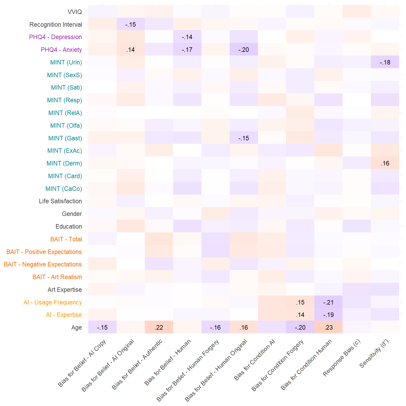
r <- dffeatures |> 
  correlation::correlation(df2, p_adjust="none") |> 
  correlation::cor_sort() |>
  mutate(label = ifelse(p < .05, paste0(insight::format_value(r, lead_zero = FALSE, zap_small = TRUE)), ""),
         Parameter1 = cleanlabels(Parameter1),
         Parameter2 = cleanlabels(Parameter2))
r[as.character(r$Parameter1) == as.character(r$Parameter2), "label"] <- ""

xnames <- levels(r$Parameter1)
ynames <- levels(r$Parameter2)

xcol <- case_when(
  str_detect(xnames, "MINT") ~ "#00838F",
  str_detect(xnames, "BAIT") ~ "#EF6C00",
  str_detect(xnames, "AI -") ~ "#FF9800",
  str_detect(xnames, "PHQ4") ~ "#9C27B0",
  str_detect(xnames, "BPQ") ~ "#795548",
  .default = "#424242"
)
ycol <- case_when(
  str_detect(ynames, "MINT") ~ "#00838F",
  str_detect(ynames, "BAIT") ~ "#EF6C00",
  str_detect(ynames, "AI -") ~ "#FF9800",
  str_detect(ynames, "PHQ4") ~ "#9C27B0",
  str_detect(ynames, "BPQ") ~ "#795548",
  .default = "#424242"
)
xbold <- case_when(
  xnames %in% c("Awareness", "MINT - Awareness") ~ "bold",
  str_detect(xnames, "Visceroception") ~ "bold",
  str_detect(xnames, "Deficit") ~ "bold",
  .default = "plain"
)
ybold <- case_when(
  ynames %in% c("Awareness", "MINT - Awareness") ~ "bold",
  str_detect(ynames, "Visceroception") ~ "bold",
  str_detect(ynames, "Deficit") ~ "bold",
  .default = "plain"
)

r |>
  ggplot(aes(x=Parameter1, y=Parameter2, fill=r)) +
  geom_tile() +
  geom_text(aes(label=label), size=3) +
  scale_fill_gradient2(low="blue", high="red", mid="white", midpoint=0, limits = c(-1, 1)) +
  theme_minimal() +
  theme(axis.text.x = element_text(angle = 45, hjust=1, color = xcol, face = xbold),
        axis.text.y = element_text(color = ycol, face = ybold),
        legend.position = "none",
        axis.title = element_blank())

Warning: Vectorized input to `element_text()` is not officially supported.
ℹ Results may be unexpected or may change in future versions of ggplot2.
Vectorized input to `element_text()` is not officially supported.
ℹ Results may be unexpected or may change in future versions of ggplot2.