Stimuli Selection

library(tidyverse)
library(ggside)
library(ggimage)

# Local path
filepaths <- list.files("C:/Users/domma/Box/Databases/Art/VAPS/VAPS/", 
                        pattern=".jpg$", full.names = TRUE, recursive = TRUE, ignore.case = TRUE) 

df <- haven::read_sav("VAPS_ValidationData.sav") |> # File provided in the database
  full_join(readxl::read_xlsx("VAPS_Information.xlsx"), by = "Picture_Number") |> 
  mutate(
    Picture_Number = as.numeric(Picture_Number),
    Folder = case_when(
      Category == 1 ~ "1 Scenes",
      Category == 2 ~ "2 Portraits",
      Category == 3 ~ "3 Landscapes",
      Category == 4 ~ "4 Still Lifes",
      .default = "5 Toward Abstraction"),
    Category = case_when(
      Category == 1 ~ "Scene",
      Category == 2 ~ "Portrait",
      Category == 3 ~ "Landscape",
      Category == 4 ~ "Still Life",
      .default = "Abstract"),
    File = paste0(Picture_Number, ".jpg"),
    Date = sub("-.*", "", Date),
    Date = sub("/.*", "", Date),
    Date = sub("ca. ", "", Date),
    Date = sub("about ", "", Date),
    Date = sub("around ", "", Date),
    Date = sub("before ", "", Date),
    Date = sub("after ", "", Date),
    Date = sub("er", "", Date),
    Date = sub("s", "", Date),
    Date = sub("um ", "", Date),
    Date = ifelse(Date %in% c("unknown", "unkown","undated", "Unknown"), NA, Date),
    Date = as.numeric(Date)) |> 
  filter(Picture_Number != "10319")  # Recognized by most members of team and pilots

df$File <- unlist(sapply(df$File, function(f) filepaths[grepl(f, filepaths, ignore.case = T)], USE.NAMES = F))

df |> 
  summarize(n = n(), .by = c("Category", "Style")) |> 
  pivot_wider(names_from = Category, values_from = n, values_fill = 0) |> 
  full_join(summarize(df, Date = paste0(min(Date, na.rm = TRUE), "-", max(Date, na.rm = TRUE)), .by = "Style"), by = "Style") |>
  gt::gt()

Style	Scene	Portrait	Landscape	Still Life	Abstract	Date
Renaissance and Mannerism	45	33	0	0	0	1434-1610
Baroque and Rococo	51	33	27	34	0	1504-1789
Idealistic tendencies	27	14	11	13	0	1781-1876
Realistic tendencies I. (19th century)	12	5	18	7	0	1821-1888
Impressionistic tendencies	15	9	13	9	0	1869-1927
Postimpressionistic tendencies	50	26	39	20	0	1852-1998
Expressionistic tendencies	31	22	28	16	8	1905-1988
Cubistic tendencies	15	10	8	15	33	1907-1937
Realistic tendencies II. (20th century)	31	31	20	26	16	1848-2012
Surrealistic tendencies	27	7	10	10	15	1911-1983
Constructivist tendencies	0	0	0	0	44	1915-1984
Informel tendencies	0	0	0	0	25	1946-1991
Abstract expressionistic tendencies	0	0	0	0	39	1930-1993

Summary

To ensure a diverse and balanced set of emotional stimuli across artistic styles, we first reclassified the original painting styles into four broader and more evenly distributed categories - “Abstract and Avant-garde”, “Impressionist and Expressionist”, “Classical”, and “Romantic and Realism” - based on shared historical and aesthetic characteristics. We then restricted selection to unfamiliar items (i.e., those rated below the median familiarity score of 1.65/7). To maximize orthogonal variability across arousal and valence, we stratified the paintings within each style into four quadrants defined by tertiles of arousal and valence, and selected the four paintings most distant from the median point (using Manhattan distance) within each quadrant. This resulted in a final set of 64 paintings (16 per style).

Style Reclassification

df$Subcategory <- df$Style

df$Style <- case_when(
  df$Style %in% c("Surrealistic tendencies", "Cubistic tendencies") | df$Category == "Abstract" ~ "Abstract and Avant-garde",
  df$Style %in% c("Impressionistic tendencies", "Postimpressionistic tendencies",
                  "Expressionistic tendencies") ~ "Impressionist and Expressionist",
  df$Style %in% c("Renaissance and Mannerism", "Baroque and Rococo") ~ "Classical",
  df$Style %in% c("Idealistic tendencies", "Realistic tendencies I. (19th century)",
                  "Realistic tendencies II. (20th century)") ~ "Romantic and Realism",
  .default = df$Style
)

df |> 
  summarize(n = n(), .by = c("Category", "Style")) |> 
  pivot_wider(names_from = Category, values_from = n, values_fill = 0) |> 
  full_join(summarize(df, N = n(), Date = paste0(min(Date, na.rm = TRUE), "-", max(Date, na.rm = TRUE)), .by = "Style"), by = "Style") |>
  gt::gt()

Style	Scene	Portrait	Landscape	Still Life	Abstract	N	Date
Classical	96	66	27	34	0	223	1434-1789
Romantic and Realism	70	50	49	46	0	215	1781-2012
Impressionist and Expressionist	96	57	80	45	0	278	1852-1998
Abstract and Avant-garde	42	17	18	25	180	282	1907-2000

Familiarity

df |> 
  ggplot(aes(x = Familarity_Mean_All)) +
  geom_histogram(bins = 50) +
  geom_vline(xintercept = median(df$Familarity_Mean_All), linetype = "dashed", color = "red") +
  theme_minimal()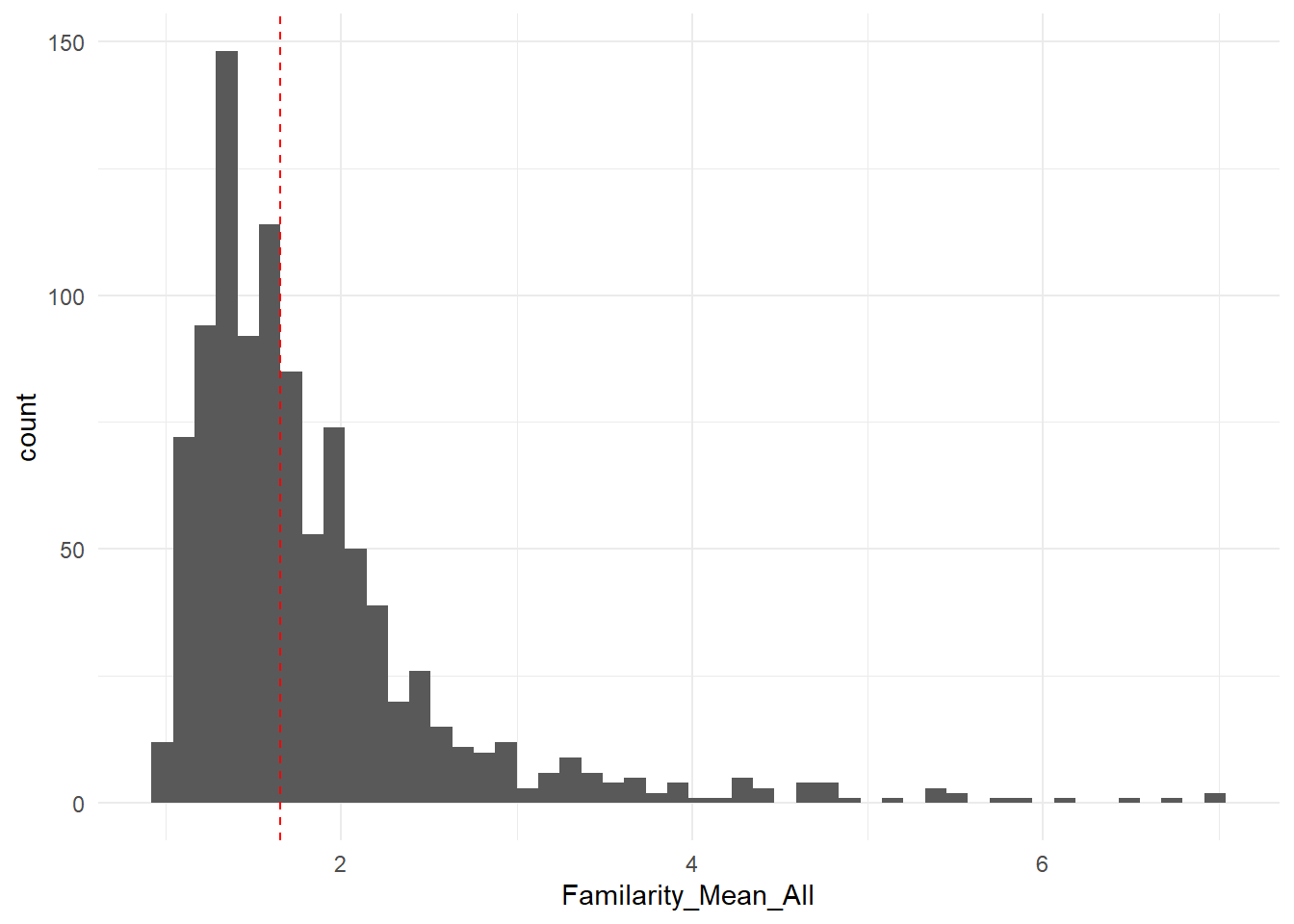

df$Familiar <- ifelse(df$Familarity_Mean_All > median(df$Familarity_Mean_All), TRUE, FALSE)

Appraisals

df |> 
  select(Picture_Number, Category, Style, Familiar,
         Liking_Mean_All, Valence_Mean_All, Arousal_Mean_All,
         Liking_Mean_Female, Valence_Mean_Female, Arousal_Mean_Female,
         Liking_Mean_Male, Valence_Mean_Male, Arousal_Mean_Male) |> 
  pivot_longer(-c(Picture_Number, Category, Style, Familiar)) |> 
  separate(name, c("Dimension", "Index", "Sex")) |> 
  pivot_wider(names_from = Dimension, values_from = value) |>
  filter(Sex == "All") |> 
  ggplot(aes(x=Valence, y=Arousal)) +
  geom_point(aes(shape = Familiar, color = Style, size = Liking), alpha = 0.8) +
  # facet_wrap(~Sex) +
  scale_shape_manual(values = c(16, 4)) +
  ggside::geom_ysidedensity(aes(linetype = Familiar)) +
  ggside::geom_xsidedensity(aes(linetype = Familiar)) +
  theme_minimal()

Warning: `is.ggproto()` was deprecated in ggplot2 3.5.2.
ℹ Please use `is_ggproto()` instead.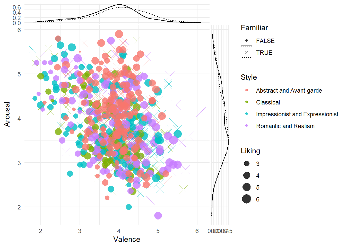

Filtering

Selection

N_per_quadrant <- 3

dffinal <- data.frame()  # Initialize selected items
dffiltered <- filter(df, Familiar == FALSE)
for(s in unique(dffiltered$Style)) {
  dat <- filter(dffiltered, Style == s)
  
  # Compute medians for quadrant splitting
  med_arousal <- median(dat$Arousal_Mean_All, na.rm = TRUE)
  med_valence <- median(dat$Valence_Mean_All, na.rm = TRUE)

  # Assign quadrant
  dat <- dat |> 
    mutate(
      Quadrant = case_when(
        Arousal_Mean_All >= quantile(Arousal_Mean_All, 2/3) & Valence_Mean_All >= quantile(Valence_Mean_All, 2/3) ~ "HA_HV",
        Arousal_Mean_All >= quantile(Arousal_Mean_All, 2/3) & Valence_Mean_All <=  quantile(Valence_Mean_All, 1/3) ~ "HA_LV",
        Arousal_Mean_All <=  quantile(Arousal_Mean_All, 1/3) & Valence_Mean_All >= quantile(Valence_Mean_All, 2/3) ~ "LA_HV",
        Arousal_Mean_All <=  quantile(Arousal_Mean_All, 1/3) & Valence_Mean_All <=  quantile(Valence_Mean_All, 1/3) ~ "LA_LV",
        .default = "Middle"
      )
    )
  
  # For each quadrant, select N items farthest from the median point
  dffinal <- dat |> 
    filter(Quadrant != "Middle") |>
    group_by(Quadrant) |> 
    mutate(
      # Euclidean distance
      # distance = sqrt((Arousal_Mean_All - med_arousal)^2 + (Valence_Mean_All - med_valence)^2)
      # Manhattan distance
      distance = abs(Arousal_Mean_All - med_arousal) + abs(Valence_Mean_All - med_valence)
    )  |> 
    slice_max(order_by = distance, n = N_per_quadrant, with_ties = FALSE)  |> 
    ungroup() |> 
    rbind(dffinal) 
}

Code

# q <- 0.78  # Quantile (adjust so to meet target N of stimuli)
# 
# dffiltered <- df |>
#   filter(Familiar == FALSE) |>
#   mutate(Liking_Up = quantile(Liking_Mean_All, q, na.rm = TRUE),
#          Liking_Down = quantile(Liking_Mean_All, 1 - q, na.rm = TRUE),
#          Arousal_Up = quantile(Arousal_Mean_All, q, na.rm = TRUE),
#          Arousal_Down = quantile(Arousal_Mean_All, 1 - q, na.rm = TRUE),
#          Valence_Up = quantile(Valence_Mean_All, q, na.rm = TRUE),
#          Valence_Down = quantile(Valence_Mean_All, 1 - q, na.rm = TRUE),
#          .by = "Style") |>
#   mutate(Liking_Extreme = ifelse(Liking_Mean_All >= Liking_Up |Liking_Mean_All <= Liking_Down, TRUE, FALSE),
#          Arousal_Extreme = ifelse(Arousal_Mean_All >= Arousal_Up | Arousal_Mean_All <= Arousal_Down, TRUE, FALSE),
#          Valence_Extreme = ifelse(Valence_Mean_All >= Valence_Up | Valence_Mean_All <= Valence_Down, TRUE, FALSE),
#          Total_Extreme = ifelse(Liking_Extreme & Arousal_Extreme & Valence_Extreme, TRUE, FALSE))
# 
# dffinal <- filter(dffiltered, Total_Extreme == TRUE)

Results

dffiltered |>
  select(Picture_Number, Category, Style,
         Liking_Mean_All, Valence_Mean_All, Arousal_Mean_All,
         Liking_Mean_Female, Valence_Mean_Female, Arousal_Mean_Female,
         Liking_Mean_Male, Valence_Mean_Male, Arousal_Mean_Male) |>
  pivot_longer(-c(Picture_Number, Category, Style)) |>
  separate(name, c("Dimension", "Index", "Sex")) |>
  pivot_wider(names_from = Dimension, values_from = value) |>
  filter(Sex == "All") |>
  mutate(Selected = as.factor(Picture_Number %in% dffinal$Picture_Number)) |> 
  ggplot(aes(x=Valence, y=Arousal)) +
  geom_point(aes(shape = Selected, color = Style, size = Liking), alpha = 0.8) +
  # facet_wrap(~Sex) +
  scale_shape_manual(values = c(4, 16)) +
  ggside::geom_ysidedensity(aes(linetype = Selected)) +
  ggside::geom_xsidedensity(aes(linetype = Selected)) +
  theme_minimal()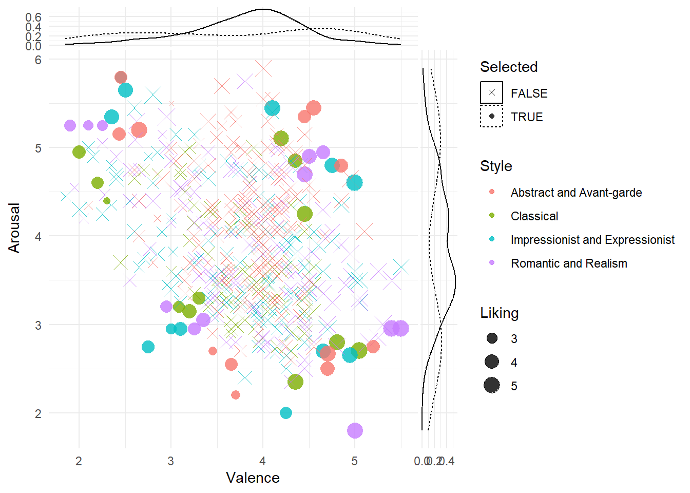

dffinal |>
  summarize(n = n(), .by = c("Style")) |> 
  rbind(data.frame(Style = "Total", n = nrow(dffinal))) |>  
  gt::gt()

Style	n
Abstract and Avant-garde	12
Impressionist and Expressionist	12
Romantic and Realism	12
Classical	12
Total	48

dat <- dffinal |> 
  select(Picture_Number, Style, File,  
         Quadrant,
         # Arousal_Up, Arousal_Down, Valence_Up, Valence_Down,
         Liking_Mean_All, Valence_Mean_All, Arousal_Mean_All,
         Liking_Mean_Female, Valence_Mean_Female, Arousal_Mean_Female,
         Liking_Mean_Male, Valence_Mean_Male, Arousal_Mean_Male) |> 
  pivot_longer(-c(Picture_Number, Style, File,
                  Quadrant)) |> 
                  # Arousal_Up, Arousal_Down, Valence_Up, Valence_Down)) |> 
  separate(name, c("Dimension", "Index", "Sex")) |> 
  pivot_wider(names_from = Dimension, values_from = value) |>
  filter(Sex == "All") |> 
  mutate(
    x_repelled = case_when(
      Quadrant == "LA_LV" ~ 0.75, 
      Quadrant == "LA_HV" ~ Valence,
      Quadrant == "HA_HV" ~ 6.5,
      Quadrant == "HA_LV"~ Valence,
      .default = Valence),
    y_repelled = case_when(
      Quadrant == "LA_LV" ~ Arousal, 
      Quadrant == "LA_HV" ~ 0.5,
      Quadrant == "HA_HV" ~ Arousal,
      Quadrant == "HA_LV" ~ 7.5,
      .default = Arousal)) |> 
  # mutate(
  #   x_repelled = case_when(
  #     Valence <= Valence_Down & Arousal <= Arousal_Down ~ 0.75, 
  #     Valence <= Valence_Down & Arousal >= Arousal_Up ~ Valence,
  #     Valence >= Valence_Up & Arousal >= Arousal_Up ~ 6.5,
  #     Valence >= Valence_Up & Arousal <= Arousal_Down ~ Valence,
  #     .default = Valence),
  #   y_repelled = case_when(
  #     Valence <= Valence_Down & Arousal <= Arousal_Down ~ Arousal, 
  #     Valence <= Valence_Down & Arousal >= Arousal_Up ~ 7,
  #     Valence >= Valence_Up & Arousal >= Arousal_Up ~ Arousal,
  #     Valence >= Valence_Up & Arousal <= Arousal_Down ~ 0.5,
  #     .default = Arousal)) |> 
  arrange(Style)



# Jitter positions
idx <- dat$Quadrant == "LA_LV"  # Left
dat$y_repelled[idx] <- seq(1.5, 6, length.out = sum(idx))
dat$x_repelled[idx] <- dat$x_repelled[idx] + rep_len(c(0, 0.5), length = sum(idx))

idx <- dat$Quadrant == "HA_LV"  # Top
dat$x_repelled[idx] <- seq(6.5, 0.75, length.out = sum(idx))
dat$y_repelled[idx] <- dat$y_repelled[idx] + rep_len(c(0, -0.5), length = sum(idx))

idx <- dat$Quadrant == "HA_HV"  # Right
dat$y_repelled[idx] <- seq(6, 1.5, length.out = sum(idx))
dat$x_repelled[idx] <- dat$x_repelled[idx] + rep_len(c(0, -0.5), length = sum(idx))

idx <- dat$Quadrant == "LA_HV"  # Bottom
dat$x_repelled[idx] <- seq(0.75, 6.5, length.out = sum(idx))
dat$y_repelled[idx] <- dat$y_repelled[idx] + rep_len(c(0, 0.5), length = sum(idx))

gc()

p <- dat |> 
  ggplot(aes(x=Valence, y=Arousal)) +
  geom_segment(aes(xend = x_repelled, yend = y_repelled, color = Style), alpha = 0.5) +
  geom_image(aes(x=x_repelled, y = y_repelled, image=File), size=0.08) +
  geom_point(aes(color = Style, size = Liking), alpha = 0.8) +
  ggside::geom_ysidedensity(aes(color = Style), linewidth = 1) +
  ggside::geom_xsidedensity(aes(color = Style), linewidth = 1) +
  theme_minimal() +
  ggside::theme_ggside_void() +
  scale_color_manual(values = c("#E41A1C", "#377EB8", "#4DAF4A", "#FF7F00")) +
  scale_size(range = c(0.5, 5), guide = "none") +
  theme(axis.title = element_text(face = "bold", size = rel(1.2)),
        legend.title = element_text(face = "bold", size = rel(1.2)))
p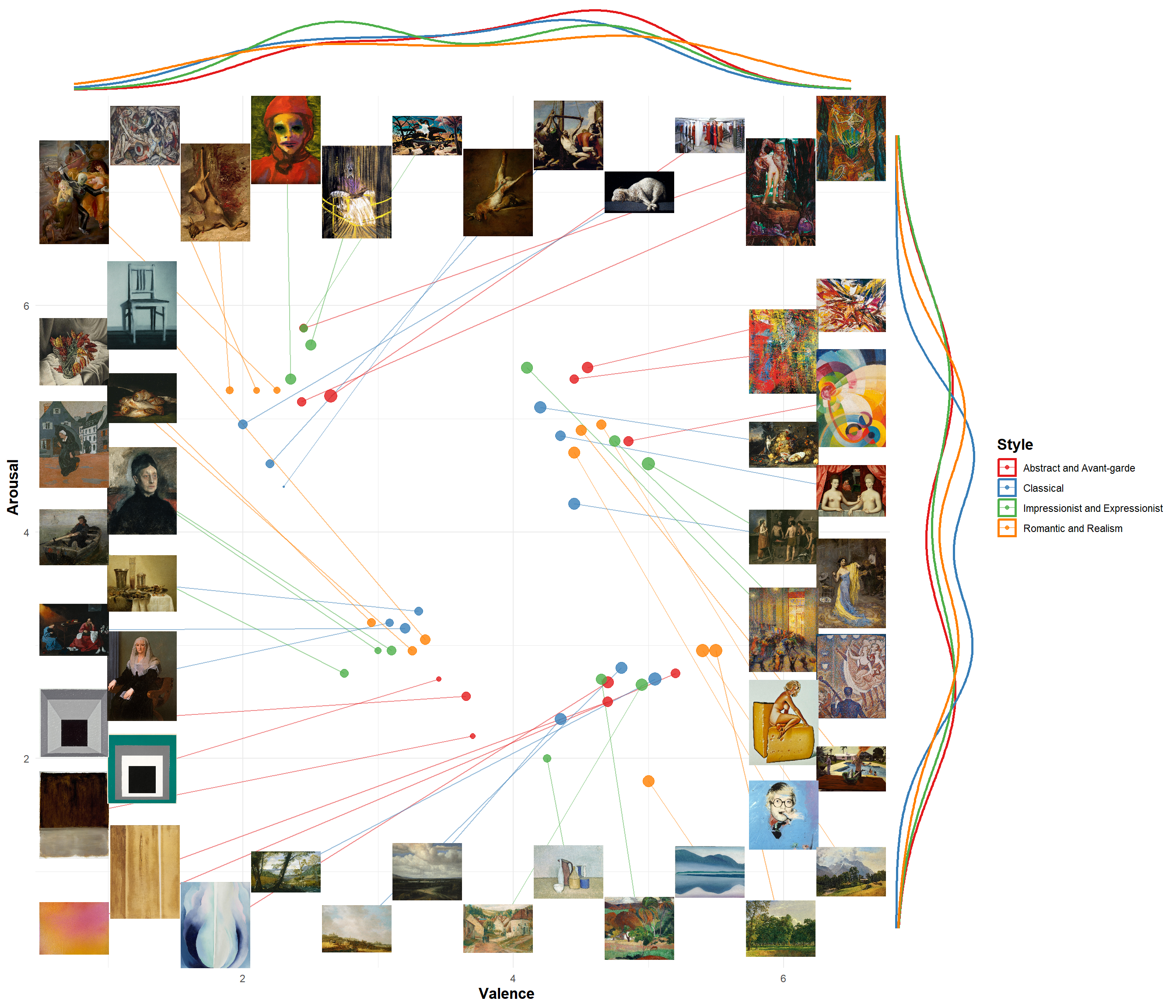

Final Selection

files <- str_split(dffinal$File, "/", simplify = TRUE)[,10]  # Change index to take last element

selection <- dffinal |> 
  mutate(Item = files) |> 
  select(Item, Category, Subcategory, Style, Artist, Title, 
         Date, Width=Width_unified, Height=Height_unified, ends_with("_All"),
         File) |> 
  arrange(Style, Item)

selection |> 
  select(-File) |> 
  gt::gt() |> 
  gt::opt_interactive() |> 
  gt::data_color(
    columns = c("Style"))|> 
  gt::data_color(
    columns = c("Liking_Mean_All", "Valence_Mean_All", "Arousal_Mean_All",
                "Complexity_Mean_All", "Familarity_Mean_All"),
    palette = c("#E41A1C", "#FF7F00", "#4DAF4A"))

Save

Code

write.csv(select(selection, -File), "../stimuli_data.csv", row.names = FALSE)

json <- selection |>
  select(Item, Style, Width, Height) |>
  jsonlite::toJSON()

write(paste("var stimuli_list = ", json), "../stimuli_list.js")

Code

# Remove all current files
unlink("../stimuli/*")

# Copy each file
for(file in selection$File) {
  file.copy(file, "../stimuli/")
}