FictionEro - Affective Impact of Fiction

Data Preparation

library(tidyverse)
library(easystats)
library(patchwork)
library(ggside)
library(glmmTMB)

options(mc.cores = parallel::detectCores(),
        brms.backend = "cmdstanr",
        width = 300)

dfsub <- read.csv("../data/data_participants.csv")
df <- read.csv("../data/data.csv") |> 
  right_join(
    select(dfsub, Participant, Sample, Language, Mobile, starts_with("Feedback_"), 
           BAIT_Visual, BAIT_Text, AI_Knowledge, SexualActivity, 
           GAAIS_Negative, GAAIS_Positive, Porn, COPS_Frequency_2,
           Screen_Size,
           -Feedback_Comments),
    by = "Participant"
    ) |> 
  datawizard::rescale(select=c("Valence"), range=c(-1, 1), to=c(0, 1)) |> 
  mutate(Condition = fct_relevel(Condition, "Photograph", "AI-Generated"),
         Relevance =  fct_relevel(Relevance, "Relevant", "Irrelevant", "Non-erotic"),
         Sex =  fct_relevel(Sex, "Male", "Female"),
         PornFrequency = as.numeric(as.factor(COPS_Frequency_2)),
         SexualActivity_num = as.numeric(as.factor(SexualActivity)),
         ConditionBelief = case_when(
           Condition == "Photograph" & Realness > 0.5 ~ "True",
           Condition == "AI-Generated" & Realness < 0.5 ~ "True",
           .default = "False"
         )) |> 
  mutate(across(starts_with("Feedback_"), function(x) {fct_relevel(x, "False", "True")}))

results_table <- function(model, effects="fixed", filter=NULL) {
  if("marginaleffects" %in% class(model)) {
    model |> 
      parameters::parameters() |> 
      as.data.frame() |> 
      select(-Parameter, -SE, -S, z=Statistic, -Predicted) |> 
      insight::format_table() |> 
      parameters::display()
  } else {
    display(parameters::parameters(model, effects=effects, keep=filter))
  }
}

Manipulation Check

This section is about selecting the best model and making a manipulation check to make sure that the emotional appraisal were sensitive to the main manipualtion (Neutral vs. Emotional).

Arousal

The Arousal data is composed of a mixture of extreme responses (0 and 1) and non-extreme responses between 0 and 1, lending itself to ordered beta model (Kubinec, 2022), designed explicitly for bounded data such as survey slider scales. It is a more parsimonious evolution of the zero-and-one inflated beta (ZOIB) regression model (see this tutorial) that jointly models the probability of extreme responses, the probability of 1 vs. 0, and the mean and spread of the rest of the responses.

arousal <- df |> 
  mutate(Arousal_Extreme = ifelse(Arousal %in% c(0, 1), "Extreme", "Not extreme")) |>
  ggplot(aes(x=Arousal, fill=Relevance)) +
  geom_histogram(aes(color=Arousal_Extreme), position = "identity", bins=80) +
  facet_grid(Relevance~Sex, scales="free_y") +
  scale_color_manual(values=c("red", "white"), guide="none") +
  scale_fill_manual(values=c("Relevant"="#E91E63", "Irrelevant"="#FF9800", "Non-erotic"="#03A9F4"), guide="none") +
  scale_y_sqrt(expand = c(0, 0)) +
  labs(title = "Arousal") +
  theme_abyss() +
  theme(plot.title = element_text(hjust = 0.5, face="bold"))

arousal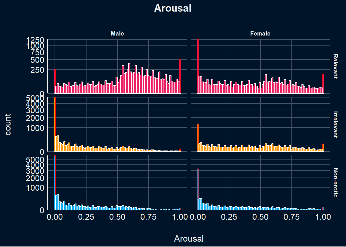

# Get a sense of Random Factors
m1 <- glmmTMB::glmmTMB(Arousal ~ Sex / Relevance + (1|Participant) + (1|Item), data=df)
m2 <- glmmTMB::glmmTMB(Arousal ~ Sex / Relevance + (1+Relevance|Participant) + (1|Item), data=df)
m3 <- glmmTMB::glmmTMB(Arousal ~ Sex / Relevance + (1|Participant) + (1+Sex|Item), data=df)
m4 <- glmmTMB::glmmTMB(Arousal ~ Sex / Relevance + (1|Participant) + (1+Relevance|Item), data=df)
m5 <- glmmTMB::glmmTMB(Arousal ~ Sex / Relevance + (1|Participant) + (1+Sex / Relevance|Item), data=df)
m6 <- glmmTMB::glmmTMB(Arousal ~ Sex / Relevance + (1+Relevance|Participant) + (1+Sex|Item), data=df)
m7 <- glmmTMB::glmmTMB(Arousal ~ Sex / Relevance + (1+Relevance|Participant) + (1+Relevance|Item), data=df)


rbind(
  mutate(performance::icc(m1, by_group=TRUE), Model = "m1"),
  data.frame(Group = "Conditional R2", ICC = performance::r2(m1)$R2_conditional, Model = "m1"),
  mutate(performance::icc(m2, by_group=TRUE), Model = "m2"),
  data.frame(Group = "Conditional R2", ICC = performance::r2(m2)$R2_conditional, Model = "m2"),
  mutate(performance::icc(m3, by_group=TRUE), Model = "m3"),
  data.frame(Group = "Conditional R2", ICC = performance::r2(m3)$R2_conditional, Model = "m3"),
  mutate(performance::icc(m4, by_group=TRUE), Model = "m4"),
  data.frame(Group = "Conditional R2", ICC = performance::r2(m4)$R2_conditional, Model = "m4"),
  mutate(performance::icc(m5, by_group=TRUE), Model = "m5"),
  data.frame(Group = "Conditional R2", ICC = performance::r2(m5)$R2_conditional, Model = "m5"),
  mutate(performance::icc(m6, by_group=TRUE), Model = "m6"),
  data.frame(Group = "Conditional R2", ICC = performance::r2(m6)$R2_conditional, Model = "m6"),
  mutate(performance::icc(m7, by_group=TRUE), Model = "m7"),
  data.frame(Group = "Conditional R2", ICC = performance::r2(m7)$R2_conditional, Model = "m7")
) |>
  ggplot(aes(x = Model, y = ICC, color=Group)) +
  geom_line(aes(group=Group))

test_bf(m6, m1, m2, m3, m4, m5, m7)
compare_performance(m2, m7)

# It seems like the full model, with the effect of relevance on participants and items, is the best.

This model evaluates the effects of Sex and Relevance on Arousal, accounting for random variability due to participants and items (i.e., random effects).

The analysis revealed that on average women rate relevant stimuli lower in arousal compared to men. Additionally, both genders tend to rate irrelevant and non-erotic stimuli lower in arousal then relevant stimuli, with males showing a stronger reduction for irrelevant stimuli and a comparable one for non-erotic stimuli. Furthermore, females rate irrelevant stimuli higher in arousal than males, whereas both genders rate non-erotic images similarly in terms of arousal.

There is notable variability in arousal ratings across participants, with a greater diversity in responses to irrelevant stimuli compared to relevant ones.There is a strong positive correlation between changes in arousal ratings for irrelevant stimuli and non-erotic stimuli. This suggests that participants who exhibit significant increases or decreases in arousal when exposed to irrelevant stimuli tend to exhibit similar changes when exposed to non-erotic stimuli, indicating consistent trends in arousal levels. There is significant variability in baseline arousal ratings across different items, indicating that different items elicit varying baseline levels of arousal.

m_a <- glmmTMB::glmmTMB(Arousal ~ Sex / Relevance + (Relevance | Participant) + (1|Item),
                      data=df, family=glmmTMB::ordbeta(),
                      control = glmmTMB::glmmTMBControl(parallel = 8))
                      # control = glmmTMB::glmmTMBControl(optimizer=stats::optim, # nlminb, optim
                      #                                   optArgs = list(method = "BFGS"),  #Nelder-Mead, BFGS, CG
                      #                                   parallel = 8))

results_table(m_a)

Fixed Effects

Parameter	Coefficient	SE	95% CI	z	p
(Intercept)	0.53	0.09	(0.36, 0.70)	6.18	< .001
Sex (Female)	-1.22	0.13	(-1.47, -0.97)	-9.63	< .001
Sex (Male) × RelevanceIrrelevant	-3.62	0.13	(-3.88, -3.35)	-26.80	< .001
Sex (Female) × RelevanceIrrelevant	-0.29	0.15	(-0.58, -5.00e-03)	-1.99	0.046
Sex (Male) × RelevanceNon-erotic	-3.66	0.13	(-3.91, -3.41)	-28.66	< .001
Sex (Female) × RelevanceNon-erotic	-2.28	0.14	(-2.56, -2.01)	-16.34	< .001

estimate_relation(m_a) |> 
  ggplot(aes(x=Relevance, y=Predicted)) +
  geom_pointrange(aes(ymin=CI_low, ymax=CI_high, color=Relevance), position=position_dodge(width=0.5)) +
  scale_color_manual(values=c("Relevant"="#E91E63", "Irrelevant"="#FF9800", "Non-erotic"="#03A9F4"), guide="none") +
  labs(y="Arousal") +
  facet_wrap(~Sex) +
  theme_abyss()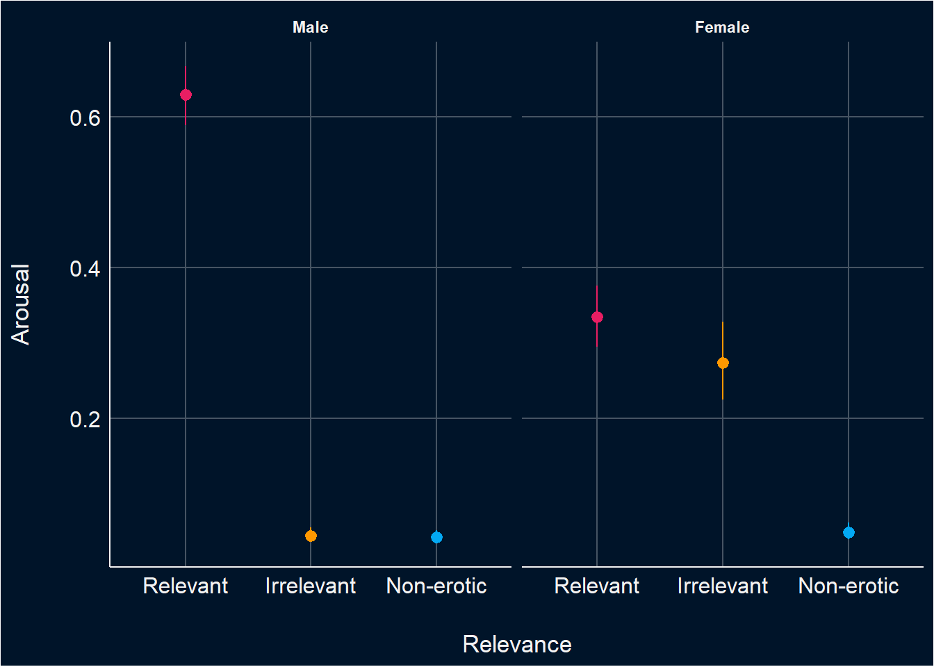

Enticement

The same type of model seems warranted for enticement.

enticiment <- df |> 
  mutate(Enticement_Extreme = ifelse(Enticement %in% c(0, 1), "Extreme", "Not extreme")) |>
  ggplot(aes(x=Enticement, fill=Relevance)) +
  geom_histogram(aes(color=Enticement_Extreme), position = "identity", bins=80) +
  facet_grid(Relevance~Sex, scales="free_y") +
  scale_color_manual(values=c("red", "white"), guide="none") +
  scale_fill_manual(values=c("Relevant"="#E91E63", "Irrelevant"="#FF9800", "Non-erotic"="#03A9F4"), guide="none") +
  scale_y_sqrt(expand = c(0, 0)) +
  labs(title = "Enticement") +
  theme_abyss() +
  theme(plot.title = element_text(hjust = 0.5, face="bold"))

enticiment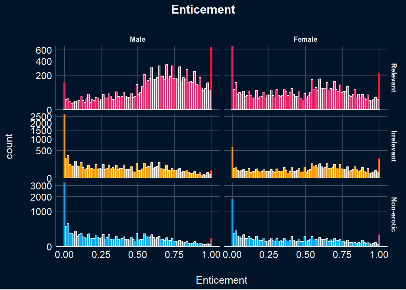

This model evaluates the effects of Sex and Relevance on Enticement ratings, accounting for random variability due to participants and items (i.e., random effects).

In general, women rate relevant images lower in enticement than males. Males rate irrelevant images significantly less enticing than relevant ones, while females do not show a significant difference in enticement ratings between irrelevant and relevant images. Both males and females rate non-erotic images as the least enticing, with a stronger effect for males.

Random effects show considerable participant-to-participant variation in baseline enticement ratings, especially for irrelevant and non-erotic stimuli, compared to relevant stimuli.Participants with higher initial ratings for relevant stimuli tend to show less change in ratings for irrelevant and non-erotic stimuli, though the effect size varies.A notable correlation exists between changes in enticement ratings for irrelevant and non-erotic stimuli, indicating consistent responsiveness across different stimulus types. Lastly, the analysis indicates that different items elicit varying baseline levels of enticement.

m_e <- glmmTMB::glmmTMB(Enticement ~ Sex / Relevance + (Relevance | Participant) + (1|Item),
                      data=df, family=glmmTMB::ordbeta(),
                      control = glmmTMB::glmmTMBControl(parallel = 8))

results_table(m_e)

Fixed Effects

Parameter	Coefficient	SE	95% CI	z	p
(Intercept)	0.79	0.08	(0.64, 0.94)	10.10	< .001
Sex (Female)	-0.94	0.11	(-1.16, -0.72)	-8.23	< .001
Sex (Male) × RelevanceIrrelevant	-2.21	0.12	(-2.45, -1.97)	-18.13	< .001
Sex (Female) × RelevanceIrrelevant	0.04	0.13	(-0.23, 0.30)	0.26	0.794
Sex (Male) × RelevanceNon-erotic	-2.42	0.12	(-2.65, -2.19)	-20.39	< .001
Sex (Female) × RelevanceNon-erotic	-1.17	0.13	(-1.42, -0.92)	-9.00	< .001

estimate_relation(m_e) |> 
  ggplot(aes(x=Relevance, y=Predicted)) +
  geom_pointrange(aes(ymin=CI_low, ymax=CI_high, color=Relevance), position=position_dodge(width=0.5)) +
  scale_color_manual(values=c("Relevant"="#E91E63", "Irrelevant"="#FF9800", "Non-erotic"="#03A9F4"), guide="none") +
  labs(y="Enticement") +
  facet_wrap(~Sex) +
  theme_abyss()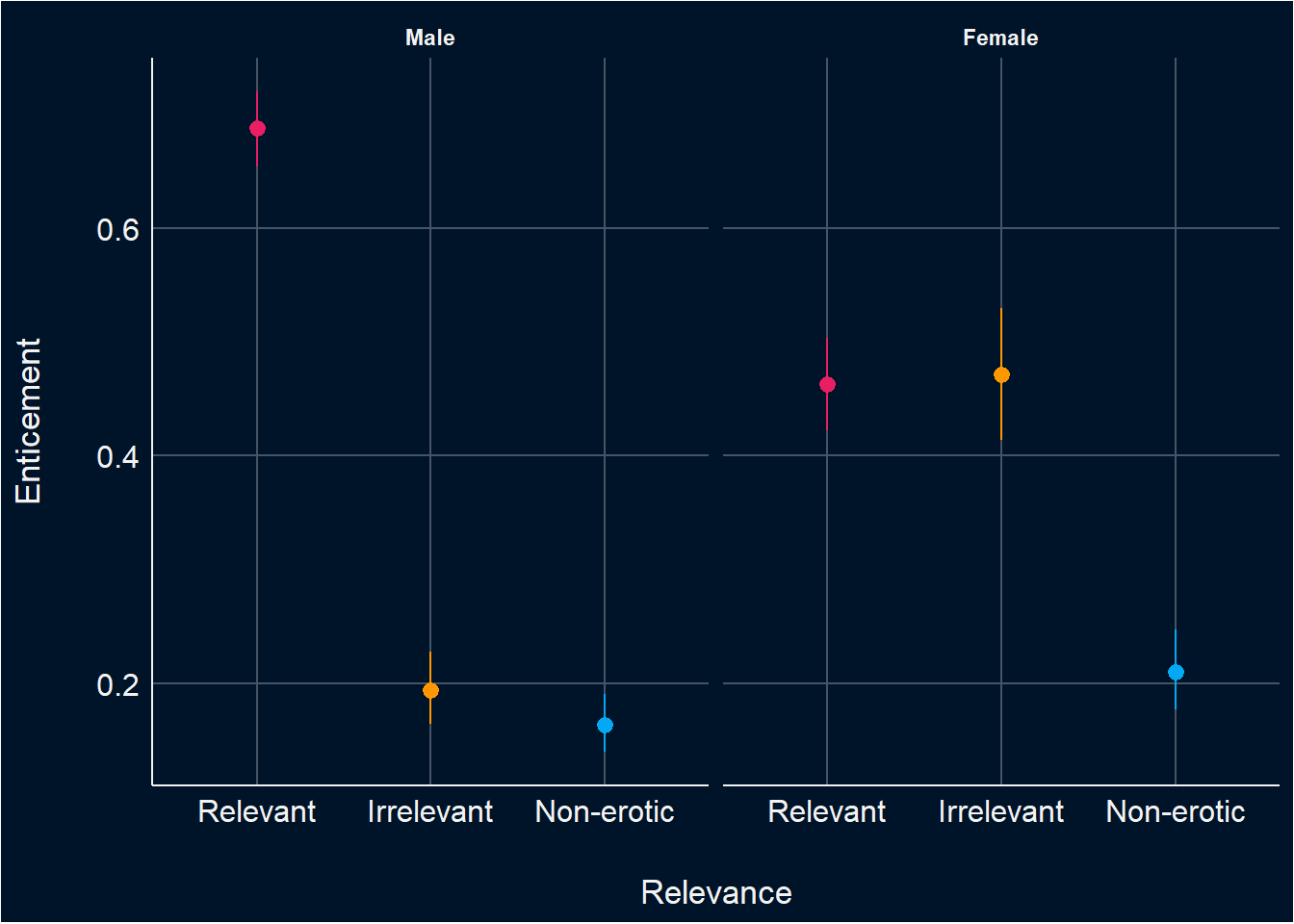

Valence

The same type of model seems warranted for valence.

valence <- df |> 
  mutate(Valence_Extreme = ifelse(Valence %in% c(0, 1), "Extreme", "Not extreme")) |>
  ggplot(aes(x=Valence, fill=Relevance)) +
  geom_histogram(aes(color=Valence_Extreme), position = "identity", bins=80) +
  facet_grid(Relevance~Sex, scales="free_y") +
  scale_color_manual(values=c("red", "white"), guide="none") +
  scale_fill_manual(values=c("Relevant"="#E91E63", "Irrelevant"="#FF9800", "Non-erotic"="#03A9F4"), guide="none") +
  scale_y_sqrt(expand = c(0, 0)) +
  labs(title = "Valence") +
  theme_abyss() +
  theme(plot.title = element_text(hjust = 0.5, face="bold"))

valence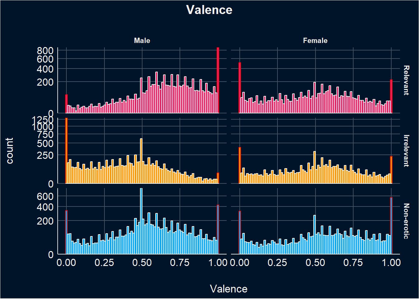

This model is evaluating the effects of Sex and Relevance on Valence ratings, accounting for random variability due to participants and items (i.e., random effects).

The analysis reveals that women rate relevant stimuli significantly lower in valence compared to men. Male participants consistently rate relevant stimuli higher in valence compared to their ratings of irrelevant stimuli, while females do not show significant differences between these stimuli. Both genders rate non-erotic stimuli lower in valence than relevant stimuli and higher than irrelevant ones, with males showing a more pronounced difference.

Participants show diverse baseline valence ratings, especially for irrelevant and non-erotic stimuli, with greater variability observed compared to relevant stimuli. Participants who rate relevant stimuli higher in valence exhibit less change in valence ratings for irrelevant and non-erotic stimuli, indicating consistent individual responses across different types of stimuli.There is a significant correlation between changes in valence ratings for irrelevant and non-erotic stimuli, indicating consistent responsiveness across different stimulus types. Different items elicit varying baseline levels of valence..

m_v <- glmmTMB::glmmTMB(Valence ~ Sex / Relevance + (Relevance | Participant) + (1|Item),
                      data=df, family=glmmTMB::ordbeta(),
                      control = glmmTMB::glmmTMBControl(parallel = 8))

results_table(m_v)

Fixed Effects

Parameter	Coefficient	SE	95% CI	z	p
(Intercept)	0.85	0.09	(0.68, 1.02)	9.89	< .001
Sex (Female)	-0.96	0.13	(-1.21, -0.71)	-7.67	< .001
Sex (Male) × RelevanceIrrelevant	-1.66	0.12	(-1.90, -1.41)	-13.34	< .001
Sex (Female) × RelevanceIrrelevant	0.04	0.13	(-0.22, 0.29)	0.28	0.781
Sex (Male) × RelevanceNon-erotic	-0.66	0.12	(-0.89, -0.42)	-5.50	< .001
Sex (Female) × RelevanceNon-erotic	0.47	0.12	(0.23, 0.72)	3.81	< .001

estimate_relation(m_v) |> 
  ggplot(aes(x=Relevance, y=Predicted)) +
  geom_pointrange(aes(ymin=CI_low, ymax=CI_high, color=Relevance), position=position_dodge(width=0.5)) +
  scale_color_manual(values=c("Relevant"="#E91E63", "Irrelevant"="#FF9800", "Non-erotic"="#03A9F4"), guide="none") +
  labs(y="Valence") +
  facet_wrap(~Sex) +
  theme_abyss()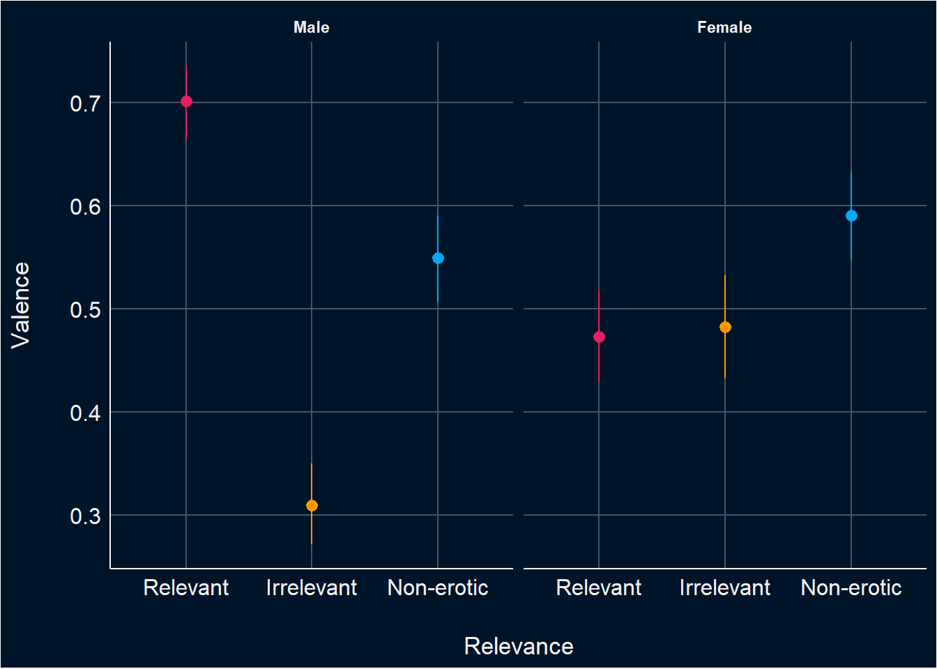

Arousal

plot_descriptive <- function(df, target="Arousal") {
  # By item
  order <- df |>
    mutate(.Item_Order = paste0(Relevance, "_", Sex, "_", Item)) |>
    summarize(mean = mean(.data[[target]], na.rm=TRUE), .by=c("Condition", ".Item_Order")) |> 
    arrange(.Item_Order, desc(Condition)) |> 
    mutate(diff = sign(mean - lag(mean)),
           Relevance = str_extract(.Item_Order, "^[^_]+"),
           .Item_Order = str_extract(.Item_Order, "(?<=_).+")) |>
    filter(Condition == "Photograph") |> 
    arrange(Relevance, diff, mean)
    
  p1 <- df |>
    mutate(.Item_Order = paste0(Sex, "_", Item)) |>
    group_by(.Item_Order, Condition) |>
    ggdist::mean_qi(.data[[target]], .width=0.95) |>
    mutate(Sex = fct_rev(str_extract(.Item_Order, "^[^_]+"))) |>
    left_join(order[c(".Item_Order", "diff")], by=".Item_Order") |>
    mutate(.Item_Order = fct_relevel(.Item_Order, order$.Item_Order)) |>
    # mutate(.average = mean(.data[[target]]), .by="Item") |>
    # mutate(Item = fct_reorder(Item, .average)) |>
    ggplot(aes(y = .Item_Order, x=.data[[target]])) +
    geom_line(aes(color=as.factor(diff)), linewidth=1) +
    geom_point(aes(color=Condition), size=2) +
      
    # ggdist::stat_slabinterval(aes(fill=Condition, color=Condition),
    #                           .width=0.95, normalize="xy", slab_alpha=0.5) +
    # ggdist::stat_histinterval(aes(fill=Condition, color=Condition),
    #                           .width=0.95, normalize="xy", slab_alpha=0.5) +
    scale_color_manual(values=c("AI-Generated"="#2196F3", "Photograph"="#F44336", "1"="#F44336", "-1"="#2196F3"),
                       breaks = c('AI-Generated', 'Photograph')) +
    # scale_fill_manual(values=c("AI-Generated"="#2196F3", "Photograph"="#F44336")) +
    scale_y_discrete(labels = function(x) str_extract(x, "(?<=_).+")) +
    theme_minimal() +
    theme(panel.grid.minor.x = element_blank(),
          # panel.grid.major.x = element_blank(),
          panel.border = element_blank(),
          axis.line.x = element_blank()) +
    labs(title = paste0(target, " by Item"), color="Condition", y="Items") +
    facet_wrap(~Sex, scales="free_y")

  # By participant
  p2 <- df |>
    summarize(.average = mean(.data[[target]]),
              .by=c("Sex", "Participant", "Condition")) |>
    pivot_wider(names_from = Condition, values_from = .average) |>
    mutate(.diff = Photograph - `AI-Generated`) |>
    mutate(Participant = fct_reorder(Participant, .diff)) |>
    ggplot(aes(x = .diff, y=Participant)) +
    geom_bar(aes(fill=.diff), stat = "identity")  +
    scale_fill_gradient2(guide="none", low="red", high="red", mid="blue") +
    labs(title = paste0(target, " by Participant")) +
    facet_wrap(~Sex, ncol=2, scales="free_y") +
    theme_minimal() +
    theme(panel.grid.major.y = element_blank(),
          panel.border = element_blank(),
          axis.line.x = element_blank(),
          axis.text.y = element_blank()) +
    labs(title = paste0(target, " by Participant"), x="Difference (Photograph - AI-Generated)", y="Participants")

  p1 / p2 + plot_layout(heights = c(2, 1))
}

arousal_desc <- plot_descriptive(df, "Arousal")
arousal_desc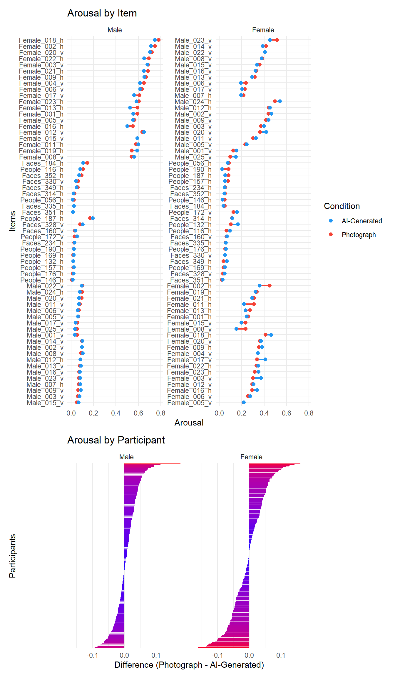

Whole Sample

This model examines the effects of Sex, Relevance, and Condition on Arousal, accounting for random variability due to participants and items (i.e., random effects).

Women rate relevant (photograph) stimuli significantly lower in arousal compared to men. Males rate irrelevant (photograph), and non-erotic (photograph), stimuli significantly lower in arousal compared to relevant stimuli. Females also rate non-erotic (photograph) stimuli lower in arousal compared to relevant stimuli. Lastly, males rate AI-Generated images significantly lower in arousal compared to Photograph images.

The analysis also examined the average marginal effect of the variable “Condition” (comparing AI-Generated to Photograph) separately for males and females. For males, the arousal is on average lower for AI-Generated images compared to Photograph images. For females, the arousal is on average higher for AI-Generated images compared to Photograph images; however, this effect is not significant.

m_arousal <- glmmTMB::glmmTMB(Arousal ~ Sex / Relevance / Condition + 
                                (Relevance | Participant) + (1|Item),
                      data=df, family=glmmTMB::ordbeta(),
                      control = glmmTMB::glmmTMBControl(parallel = 8))

results_table(m_arousal)

Fixed Effects

Parameter	Coefficient	SE	95% CI	z	p
(Intercept)	0.57	0.09	(0.40, 0.74)	6.57	< .001
Sex (Female)	-1.27	0.13	(-1.52, -1.02)	-9.98	< .001
Sex (Male) × RelevanceIrrelevant	-3.65	0.14	(-3.92, -3.39)	-26.87	< .001
Sex (Female) × RelevanceIrrelevant	-0.27	0.15	(-0.56, 0.01)	-1.86	0.063
Sex (Male) × RelevanceNon-erotic	-3.67	0.13	(-3.92, -3.42)	-28.45	< .001
Sex (Female) × RelevanceNon-erotic	-2.30	0.14	(-2.58, -2.02)	-16.22	< .001
Sex (Male) × RelevanceRelevant × ConditionAI-Generated	-0.07	0.02	(-0.11, -0.04)	-4.07	< .001
Sex (Female) × RelevanceRelevant × ConditionAI-Generated	0.03	0.03	(-0.02, 0.09)	1.29	0.197
Sex (Male) × RelevanceIrrelevant × ConditionAI-Generated	-2.67e-03	0.03	(-0.06, 0.05)	-0.10	0.924
Sex (Female) × RelevanceIrrelevant × ConditionAI-Generated	-1.20e-03	0.03	(-0.05, 0.05)	-0.05	0.964
Sex (Male) × RelevanceNon-erotic × ConditionAI-Generated	-0.06	0.03	(-0.12, 4.90e-03)	-1.81	0.071
Sex (Female) × RelevanceNon-erotic × ConditionAI-Generated	0.07	0.04	(-0.01, 0.15)	1.68	0.094

marginaleffects::avg_slopes(m_arousal, variables="Condition", by="Sex", re.form=NA) |> 
  results_table()

Comparison	Sex	Coefficient	z	p	95% CI	predicted_lo	predicted_hi
mean(AI-Generated) - mean(Photograph)	Male	-6.60e-03	-4.28	< .001	[-0.01, 0.00]	0.04	0.04
mean(AI-Generated) - mean(Photograph)	Female	3.48e-03	1.29	0.197	[ 0.00, 0.01]	0.33	0.34

Subsamples

Sample

When examining the random slopes, it was observed that only males significantly rated arousal lower for AI-generated images compared to photographs. Further analysis of the sample subgroups revealed that this effect was predominantly driven by males from the general population, who significantly contributed to the lower arousal ratings for AI-generated images compared to photographs.

m <- glmmTMB::glmmTMB(Arousal ~ Sample / Sex / Relevance / Condition + (Relevance | Participant) + (1|Item),
                      data=df, 
                      family=glmmTMB::ordbeta(),
                      control = glmmTMB::glmmTMBControl(parallel = 8))

results_table(m, filter="Condition")

Fixed Effects

Parameter	Coefficient	SE	95% CI	z	p
Sample (General Population) × SexMale × RelevanceRelevant × ConditionAI-Generated	-0.08	0.02	(-0.12, -0.04)	-3.84	< .001
Sample (Students (Incentivized)) × SexMale × RelevanceRelevant × ConditionAI-Generated	-0.07	0.06	(-0.19, 0.04)	-1.23	0.220
Sample (Students (Non-incentivized)) × SexMale × RelevanceRelevant × ConditionAI-Generated	-0.04	0.06	(-0.16, 0.07)	-0.79	0.432
Sample (General Population) × SexFemale × RelevanceRelevant × ConditionAI-Generated	0.06	0.05	(-0.04, 0.15)	1.18	0.238
Sample (Students (Incentivized)) × SexFemale × RelevanceRelevant × ConditionAI-Generated	-0.01	0.04	(-0.10, 0.07)	-0.26	0.792
Sample (Students (Non-incentivized)) × SexFemale × RelevanceRelevant × ConditionAI-Generated	0.06	0.04	(-0.03, 0.15)	1.38	0.169
Sample (General Population) × SexMale × RelevanceIrrelevant × ConditionAI-Generated	3.64e-03	0.03	(-0.06, 0.06)	0.12	0.904
Sample (Students (Incentivized)) × SexMale × RelevanceIrrelevant × ConditionAI-Generated	-0.10	0.11	(-0.32, 0.12)	-0.88	0.381
Sample (Students (Non-incentivized)) × SexMale × RelevanceIrrelevant × ConditionAI-Generated	-4.46e-04	0.10	(-0.20, 0.20)	-4.35e-03	0.997
Sample (General Population) × SexFemale × RelevanceIrrelevant × ConditionAI-Generated	0.04	0.05	(-0.05, 0.14)	0.89	0.375
Sample (Students (Incentivized)) × SexFemale × RelevanceIrrelevant × ConditionAI-Generated	0.01	0.04	(-0.07, 0.10)	0.30	0.766
Sample (Students (Non-incentivized)) × SexFemale × RelevanceIrrelevant × ConditionAI-Generated	-0.06	0.05	(-0.15, 0.03)	-1.23	0.220
Sample (General Population) × SexMale × RelevanceNon-erotic × ConditionAI-Generated	-0.05	0.03	(-0.12, 0.02)	-1.42	0.157
Sample (Students (Incentivized)) × SexMale × RelevanceNon-erotic × ConditionAI-Generated	-0.02	0.12	(-0.26, 0.23)	-0.13	0.893
Sample (Students (Non-incentivized)) × SexMale × RelevanceNon-erotic × ConditionAI-Generated	-0.18	0.11	(-0.41, 0.04)	-1.63	0.102
Sample (General Population) × SexFemale × RelevanceNon-erotic × ConditionAI-Generated	0.08	0.08	(-0.07, 0.23)	1.07	0.284
Sample (Students (Incentivized)) × SexFemale × RelevanceNon-erotic × ConditionAI-Generated	0.03	0.07	(-0.11, 0.17)	0.48	0.634
Sample (Students (Non-incentivized)) × SexFemale × RelevanceNon-erotic × ConditionAI-Generated	0.09	0.07	(-0.04, 0.21)	1.33	0.184

Mobile

We investigated the influence of using a mobile device (mobile = TRUE) versus other devices on arousal ratings, considering the effects of condition and relevance.

Males rated relevant AI-generated images significantly lower in arousal compared to relevant photographs, irrespective of whether they used a mobile device or not. However, this effect was more pronounced among male participants who used a mobile device.

We also explored whether the interaction between condition (AI-Generated vs. Photograph) and screen size affected arousal levels. No statistically significant results were found for this interaction.

m <- glmmTMB::glmmTMB(Arousal ~ Mobile / Sex / Relevance / Condition + (Relevance | Participant) + (1|Item),
                      data=df, 
                      family=glmmTMB::ordbeta(),
                      control = glmmTMB::glmmTMBControl(parallel = 8))

results_table(m, filter="Condition")

Fixed Effects

Parameter	Coefficient	SE	95% CI	z	p
Mobile (False) × SexMale × RelevanceRelevant × ConditionAI-Generated	-0.05	0.02	(-0.09, -1.89e-03)	-2.04	0.041
Mobile (True) × SexMale × RelevanceRelevant × ConditionAI-Generated	-0.12	0.03	(-0.18, -0.06)	-4.01	< .001
Mobile (False) × SexFemale × RelevanceRelevant × ConditionAI-Generated	0.04	0.03	(-0.02, 0.10)	1.29	0.199
Mobile (True) × SexFemale × RelevanceRelevant × ConditionAI-Generated	0.02	0.05	(-0.08, 0.12)	0.37	0.714
Mobile (False) × SexMale × RelevanceIrrelevant × ConditionAI-Generated	-0.02	0.04	(-0.10, 0.06)	-0.49	0.621
Mobile (True) × SexMale × RelevanceIrrelevant × ConditionAI-Generated	0.01	0.04	(-0.06, 0.09)	0.36	0.715
Mobile (False) × SexFemale × RelevanceIrrelevant × ConditionAI-Generated	-9.93e-03	0.03	(-0.07, 0.05)	-0.32	0.748
Mobile (True) × SexFemale × RelevanceIrrelevant × ConditionAI-Generated	0.02	0.05	(-0.08, 0.13)	0.45	0.656
Mobile (False) × SexMale × RelevanceNon-erotic × ConditionAI-Generated	-0.06	0.05	(-0.15, 0.04)	-1.21	0.225
Mobile (True) × SexMale × RelevanceNon-erotic × ConditionAI-Generated	-0.06	0.04	(-0.14, 0.03)	-1.34	0.181
Mobile (False) × SexFemale × RelevanceNon-erotic × ConditionAI-Generated	0.04	0.05	(-0.06, 0.14)	0.77	0.441
Mobile (True) × SexFemale × RelevanceNon-erotic × ConditionAI-Generated	0.12	0.07	(-0.01, 0.26)	1.81	0.070

m <- glmmTMB::glmmTMB(Arousal ~ Sex / Relevance / (Condition * Screen_Size) + (Relevance | Participant) + (1|Item),
                      data=standardize(df, select="Screen_Size"), 
                      family=glmmTMB::ordbeta(),
                      control = glmmTMB::glmmTMBControl(parallel = 8))

results_table(m, filter="Screen")

Fixed Effects

Parameter	Coefficient	SE	95% CI	z	p
Sex (Male) × RelevanceRelevant × Screen Size	0.02	0.04	(-0.06, 0.10)	0.51	0.612
Sex (Female) × RelevanceRelevant × Screen Size	0.10	0.07	(-0.05, 0.24)	1.29	0.197
Sex (Male) × RelevanceIrrelevant × Screen Size	0.10	0.09	(-0.07, 0.27)	1.18	0.238
Sex (Female) × RelevanceIrrelevant × Screen Size	0.09	0.15	(-0.19, 0.38)	0.63	0.528
Sex (Male) × RelevanceNon-erotic × Screen Size	0.04	0.07	(-0.11, 0.18)	0.49	0.621
Sex (Female) × RelevanceNon-erotic × Screen Size	0.16	0.13	(-0.10, 0.41)	1.21	0.226
Sex (Male) × RelevanceRelevant × ConditionAI-Generated × Screen Size	-0.03	0.02	(-0.06, 7.04e-03)	-1.57	0.118
Sex (Female) × RelevanceRelevant × ConditionAI-Generated × Screen Size	-0.03	0.03	(-0.10, 0.04)	-0.90	0.368
Sex (Male) × RelevanceIrrelevant × ConditionAI-Generated × Screen Size	0.04	0.03	(-0.01, 0.10)	1.47	0.142
Sex (Female) × RelevanceIrrelevant × ConditionAI-Generated × Screen Size	0.04	0.03	(-0.02, 0.11)	1.27	0.205
Sex (Male) × RelevanceNon-erotic × ConditionAI-Generated × Screen Size	-0.01	0.03	(-0.08, 0.05)	-0.37	0.708
Sex (Female) × RelevanceNon-erotic × ConditionAI-Generated × Screen Size	0.08	0.05	(-0.02, 0.19)	1.56	0.118

Moderators

This model explores whether various factors such as attitudes towards AI, knowledge about AI, porn usage, frequency of porn consumption, and sexual activity moderate the relationship between sex, image relevance (specifically AI-generated versus photographs), and arousal ratings.

The analysis revealed a significant interaction effect only for porn usage among females. Specifically, females with higher levels of porn usage rated AI-generated images significantly lower in arousal compared to photographs. No other moderators showed statistically significant effects on arousal ratings across the interactions of sex, condition (AI-Generated vs. Photograph), and the respective moderators.

We also examined whether feedback moderates the relationship between sex, condition, and relevance on arousal, we found the following significant effects:

Findings suggest that feedback about the arousal potential of AI-generated images can significantly moderate arousal ratings, with females being more positively influenced by feedback that AI images are more arousing, and males being more negatively influenced by feedback that AI images are less arousing.

test_moderator <- function(df, outcome="Arousal", moderator="BAIT_Visual") {
  f <- paste0(outcome, " ~ Sex / (Condition * ", moderator, ") + (Condition | Participant) + (1|Item)")
  r <- glmmTMB::glmmTMB(as.formula(f),
                      data=filter(df, Relevance == "Relevant"), 
                      family=glmmTMB::ordbeta(),
                      control = glmmTMB::glmmTMBControl(parallel = 8)) |>
    parameters::parameters() |> 
    as.data.frame() |> 
    select(-df_error, -Effects, -Group, -Component, -SE)
  r$Moderator <- moderator
  r$Outcome <- outcome
  insight::format_table(r[c(7, 8), ])
}


moderator_results <- data.frame()
for(m in c("BAIT_Visual", "BAIT_Text", "AI_Knowledge",
           "GAAIS_Positive", "GAAIS_Negative",
           "Porn", "PornFrequency", "SexualActivity_num")) {
  moderator_results <- rbind(moderator_results,
                             test_moderator(df, "Arousal", m))
}

display(moderator_results)

Parameter	Coefficient	95% CI	z	p	Moderator	Outcome
Sex [Male] × ConditionAI-Generated × BAIT Visual	-0.11	[-0.34, 0.12]	-0.92	0.356	BAIT_Visual	Arousal
Sex [Female] × ConditionAI-Generated × BAIT Visual	0.28	[-0.12, 0.68]	1.38	0.166	BAIT_Visual	Arousal
Sex [Male] × ConditionAI-Generated × BAIT Text	-2.50e-03	[-0.16, 0.16]	-0.03	0.976	BAIT_Text	Arousal
Sex [Female] × ConditionAI-Generated × BAIT Text	0.04	[-0.24, 0.31]	0.25	0.801	BAIT_Text	Arousal
Sex [Male] × ConditionAI-Generated × AI Knowledge	0.02	[-0.01, 0.06]	1.37	0.170	AI_Knowledge	Arousal
Sex [Female] × ConditionAI-Generated × AI Knowledge	0.01	[-0.03, 0.06]	0.59	0.556	AI_Knowledge	Arousal
Sex [Male] × ConditionAI-Generated × GAAIS Positive	0.08	[-0.11, 0.27]	0.84	0.398	GAAIS_Positive	Arousal
Sex [Female] × ConditionAI-Generated × GAAIS Positive	0.17	[-0.13, 0.47]	1.09	0.276	GAAIS_Positive	Arousal
Sex [Male] × ConditionAI-Generated × GAAIS Negative	-0.03	[-0.19, 0.14]	-0.31	0.759	GAAIS_Negative	Arousal
Sex [Female] × ConditionAI-Generated × GAAIS Negative	0.17	[-0.11, 0.46]	1.22	0.224	GAAIS_Negative	Arousal
Sex [Male] × ConditionAI-Generated × Porn	-0.04	[-0.09, 0.02]	-1.35	0.177	Porn	Arousal
Sex [Female] × ConditionAI-Generated × Porn	-0.08	[-0.16, 0.00]	-2.06	0.040	Porn	Arousal
Sex [Male] × ConditionAI-Generated × PornFrequency	-0.01	[-0.04, 0.01]	-0.90	0.368	PornFrequency	Arousal
Sex [Female] × ConditionAI-Generated × PornFrequency	-0.03	[-0.07, 0.02]	-1.25	0.212	PornFrequency	Arousal
Sex [Male] × ConditionAI-Generated × SexualActivity num	-2.95e-03	[-0.04, 0.03]	-0.16	0.876	SexualActivity_num	Arousal
Sex [Female] × ConditionAI-Generated × SexualActivity num	-0.01	[-0.06, 0.03]	-0.65	0.515	SexualActivity_num	Arousal

feedback_results <- data.frame()
for(m in c("Feedback_CouldDiscriminate", "Feedback_CouldNotDiscriminate",
           "Feedback_AIMoreArousing", "Feedback_AILessArousing", 
           "Feedback_LabelsIncorrect", "Feedback_LabelsReversed")) {
  feedback_results <- rbind(feedback_results,
                            test_moderator(df, "Arousal", m))
}
display(feedback_results)

Parameter	Coefficient	95% CI	z	p	Moderator	Outcome
Sex [Male] × ConditionAI-Generated × Feedback CouldDiscriminateTrue	0.06	[-0.09, 0.21]	0.80	0.421	Feedback_CouldDiscriminate	Arousal
Sex [Female] × ConditionAI-Generated × Feedback CouldDiscriminateTrue	-0.14	[-0.38, 0.10]	-1.17	0.241	Feedback_CouldDiscriminate	Arousal
Sex [Male] × ConditionAI-Generated × Feedback CouldNotDiscriminateTrue	8.61e-03	[-0.07, 0.09]	0.21	0.833	Feedback_CouldNotDiscriminate	Arousal
Sex [Female] × ConditionAI-Generated × Feedback CouldNotDiscriminateTrue	0.03	[-0.09, 0.14]	0.48	0.630	Feedback_CouldNotDiscriminate	Arousal
Sex [Male] × ConditionAI-Generated × Feedback AIMoreArousingTrue	0.02	[-0.12, 0.15]	0.23	0.821	Feedback_AIMoreArousing	Arousal
Sex [Female] × ConditionAI-Generated × Feedback AIMoreArousingTrue	0.15	[ 0.00, 0.30]	1.96	0.050	Feedback_AIMoreArousing	Arousal
Sex [Male] × ConditionAI-Generated × Feedback AILessArousingTrue	-0.14	[-0.27, -0.02]	-2.19	0.028	Feedback_AILessArousing	Arousal
Sex [Female] × ConditionAI-Generated × Feedback AILessArousingTrue	0.16	[-0.03, 0.36]	1.64	0.102	Feedback_AILessArousing	Arousal
Sex [Male] × ConditionAI-Generated × Feedback LabelsIncorrectTrue	-0.04	[-0.12, 0.04]	-0.94	0.349	Feedback_LabelsIncorrect	Arousal
Sex [Female] × ConditionAI-Generated × Feedback LabelsIncorrectTrue	-0.04	[-0.17, 0.08]	-0.70	0.485	Feedback_LabelsIncorrect	Arousal
Sex [Male] × ConditionAI-Generated × Feedback LabelsReversedTrue	-0.08	[-0.27, 0.10]	-0.89	0.371	Feedback_LabelsReversed	Arousal
Sex [Female] × ConditionAI-Generated × Feedback LabelsReversedTrue	2.95e-03	[-0.21, 0.22]	0.03	0.978	Feedback_LabelsReversed	Arousal

Believed

  m <- glmmTMB::glmmTMB(Arousal ~ Sex / Relevance / Condition + (Relevance | Participant) + (1|Item),
                        data=filter(df, ConditionBelief == "True"), 
                        family=glmmTMB::ordbeta(),
                        control = glmmTMB::glmmTMBControl(parallel = 8))
  
  results_table(m)

Fixed Effects

Parameter	Coefficient	SE	95% CI	z	p
(Intercept)	0.62	0.09	(0.45, 0.79)	7.29	< .001
Sex (Female)	-1.17	0.13	(-1.42, -0.92)	-9.27	< .001
Sex (Male) × RelevanceIrrelevant	-3.64	0.14	(-3.90, -3.37)	-26.72	< .001
Sex (Female) × RelevanceIrrelevant	-0.35	0.14	(-0.63, -0.06)	-2.39	0.017
Sex (Male) × RelevanceNon-erotic	-3.74	0.13	(-3.99, -3.48)	-28.47	< .001
Sex (Female) × RelevanceNon-erotic	-2.40	0.14	(-2.68, -2.11)	-16.61	< .001
Sex (Male) × RelevanceRelevant × ConditionAI-Generated	-0.38	0.03	(-0.45, -0.31)	-10.85	< .001
Sex (Female) × RelevanceRelevant × ConditionAI-Generated	-0.39	0.05	(-0.48, -0.30)	-8.43	< .001
Sex (Male) × RelevanceIrrelevant × ConditionAI-Generated	-0.07	0.05	(-0.16, 0.03)	-1.36	0.173
Sex (Female) × RelevanceIrrelevant × ConditionAI-Generated	-0.15	0.05	(-0.25, -0.06)	-3.30	< .001
Sex (Male) × RelevanceNon-erotic × ConditionAI-Generated	-0.16	0.07	(-0.30, -0.02)	-2.26	0.024
Sex (Female) × RelevanceNon-erotic × ConditionAI-Generated	-0.09	0.09	(-0.27, 0.09)	-0.95	0.340

  moderator_believed <- data.frame()
  for(m in c("BAIT_Visual", "BAIT_Text", "AI_Knowledge",
             "GAAIS_Positive", "GAAIS_Negative",
             "Porn", "PornFrequency", "SexualActivity_num", 
             "Feedback_CouldDiscriminate", "Feedback_CouldNotDiscriminate",
             "Feedback_AIMoreArousing", "Feedback_AILessArousing", 
             "Feedback_LabelsIncorrect", "Feedback_LabelsReversed")) {
    moderator_believed <- rbind(moderator_believed,
                               test_moderator(filter(df, ConditionBelief == "True"), "Arousal", m))
  }
  
  display(filter(moderator_believed, p < .1))

Parameter	Coefficient	95% CI	z	p	Moderator	Outcome
Sex [Female] × ConditionAI-Generated × GAAIS Negative	0.58	[ 0.01, 1.15]	2.01	0.045	GAAIS_Negative	Arousal
Sex [Female] × ConditionAI-Generated × Porn	-0.17	[-0.33, -0.01]	-2.10	0.036	Porn	Arousal
Sex [Female] × ConditionAI-Generated × SexualActivity num	-0.12	[-0.21, -0.04]	-2.85	0.004	SexualActivity_num	Arousal
Sex [Male] × ConditionAI-Generated × Feedback AILessArousingTrue	-0.32	[-0.54, -0.09]	-2.80	0.005	Feedback_AILessArousing	Arousal

Enticement

enticement_desc <- plot_descriptive(df, "Enticement")
enticement_desc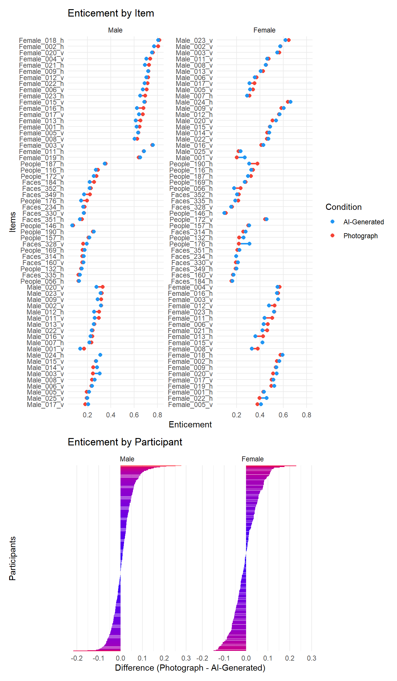

Whole Sample

This model examines how Sex, Relevance, and Condition influence Valence ratings, treating relevance within each participant and items as random effects.

Females consistently rate relevant (photograph) images significantly lower in enticement compared to males. Conversely, men rate irrelevant images (photographs) significantly lower in enticement than relevant ones, although this difference is not observed among females. Both genders rate non-erotic images (photographs) significantly lower in enticement than relevant ones. Interestingly, neither gender shows a significant difference in enticement ratings between AI-generated images and photographs, regardless of relevance.

We also analyzed the average marginal effect of the variable “Condition” (comparing AI-Generated to Photograph) separately for males and females.

For males, enticement ratings are significantly lower on average for AI-Generated images compared to Photograph images. For females, enticement ratings are slightly higher on average for AI-Generated images compared to Photograph images, although this difference is not statistically significant.

m_enticement <- glmmTMB::glmmTMB(Enticement ~ Sex / Relevance / Condition + 
                                   (Relevance | Participant) + (1|Item),
                      data=df, family=glmmTMB::ordbeta(),
                      control = glmmTMB::glmmTMBControl(parallel = 8))

results_table(m_enticement)

Fixed Effects

Parameter	Coefficient	SE	95% CI	z	p
(Intercept)	0.83	0.08	(0.68, 0.99)	10.55	< .001
Sex (Female)	-0.99	0.12	(-1.22, -0.77)	-8.62	< .001
Sex (Male) × RelevanceIrrelevant	-2.25	0.12	(-2.49, -2.01)	-18.33	< .001
Sex (Female) × RelevanceIrrelevant	0.05	0.14	(-0.21, 0.32)	0.39	0.693
Sex (Male) × RelevanceNon-erotic	-2.44	0.12	(-2.67, -2.20)	-20.37	< .001
Sex (Female) × RelevanceNon-erotic	-1.16	0.13	(-1.42, -0.91)	-8.85	< .001
Sex (Male) × RelevanceRelevant × ConditionAI-Generated	-0.08	0.02	(-0.12, -0.04)	-4.30	< .001
Sex (Female) × RelevanceRelevant × ConditionAI-Generated	0.03	0.02	(-0.02, 0.07)	1.01	0.311
Sex (Male) × RelevanceIrrelevant × ConditionAI-Generated	-2.95e-03	0.02	(-0.05, 0.04)	-0.14	0.891
Sex (Female) × RelevanceIrrelevant × ConditionAI-Generated	-0.01	0.03	(-0.06, 0.04)	-0.46	0.647
Sex (Male) × RelevanceNon-erotic × ConditionAI-Generated	-0.05	0.02	(-0.10, -6.01e-03)	-2.22	0.026
Sex (Female) × RelevanceNon-erotic × ConditionAI-Generated	0.01	0.03	(-0.05, 0.07)	0.40	0.686

marginaleffects::avg_slopes(m_enticement, variables="Condition", by="Sex", re.form=NA) |> 
  results_table()

Comparison	Sex	Coefficient	z	p	95% CI	predicted_lo	predicted_hi
mean(AI-Generated) - mean(Photograph)	Male	-8.31e-03	-4.04	< .001	[-0.01, 0.00]	0.17	0.16
mean(AI-Generated) - mean(Photograph)	Female	1.79e-03	0.53	0.596	[ 0.00, 0.01]	0.46	0.47

Subsamples

Sample

Here we examined the interaction between Sample (different participant groups), Sex, Relevance, and Condition (AI-Generated vs. Photograph) on enticement ratings.

These findings indicate that in the General Population and Students (Non-incentivized) samples, males show a preference for relevant Photograph images over relevant AI-Generated images in terms of enticement, while females tend to rate relevant AI-Generated images higher in enticement. The differences in enticement ratings between AI-Generated and Photograph images were not significant in other samples or conditions examined.

m <- glmmTMB::glmmTMB(Enticement ~ Sample / Sex / Relevance / Condition + (Relevance | Participant) + (1|Item),
                      data=df, 
                      family=glmmTMB::ordbeta(),
                      control = glmmTMB::glmmTMBControl(parallel = 8))

results_table(m, filter="Condition")

Fixed Effects

Parameter	Coefficient	SE	95% CI	z	p
Sample (General Population) × SexMale × RelevanceRelevant × ConditionAI-Generated	-0.09	0.02	(-0.13, -0.05)	-4.34	< .001
Sample (Students (Incentivized)) × SexMale × RelevanceRelevant × ConditionAI-Generated	-0.08	0.06	(-0.20, 0.05)	-1.22	0.222
Sample (Students (Non-incentivized)) × SexMale × RelevanceRelevant × ConditionAI-Generated	-6.24e-03	0.06	(-0.12, 0.11)	-0.10	0.917
Sample (General Population) × SexFemale × RelevanceRelevant × ConditionAI-Generated	0.02	0.05	(-0.08, 0.11)	0.37	0.713
Sample (Students (Incentivized)) × SexFemale × RelevanceRelevant × ConditionAI-Generated	-0.04	0.04	(-0.12, 0.04)	-1.04	0.297
Sample (Students (Non-incentivized)) × SexFemale × RelevanceRelevant × ConditionAI-Generated	0.11	0.04	(0.02, 0.19)	2.54	0.011
Sample (General Population) × SexMale × RelevanceIrrelevant × ConditionAI-Generated	-1.60e-03	0.02	(-0.05, 0.04)	-0.07	0.946
Sample (Students (Incentivized)) × SexMale × RelevanceIrrelevant × ConditionAI-Generated	-0.08	0.08	(-0.24, 0.07)	-1.04	0.299
Sample (Students (Non-incentivized)) × SexMale × RelevanceIrrelevant × ConditionAI-Generated	0.05	0.07	(-0.09, 0.19)	0.68	0.496
Sample (General Population) × SexFemale × RelevanceIrrelevant × ConditionAI-Generated	-0.03	0.05	(-0.12, 0.07)	-0.53	0.599
Sample (Students (Incentivized)) × SexFemale × RelevanceIrrelevant × ConditionAI-Generated	-0.04	0.04	(-0.12, 0.04)	-0.98	0.325
Sample (Students (Non-incentivized)) × SexFemale × RelevanceIrrelevant × ConditionAI-Generated	0.03	0.04	(-0.05, 0.12)	0.77	0.441
Sample (General Population) × SexMale × RelevanceNon-erotic × ConditionAI-Generated	-0.06	0.03	(-0.10, -5.33e-03)	-2.17	0.030
Sample (Students (Incentivized)) × SexMale × RelevanceNon-erotic × ConditionAI-Generated	0.11	0.08	(-0.05, 0.27)	1.37	0.171
Sample (Students (Non-incentivized)) × SexMale × RelevanceNon-erotic × ConditionAI-Generated	-0.14	0.07	(-0.28, -4.25e-03)	-2.02	0.043
Sample (General Population) × SexFemale × RelevanceNon-erotic × ConditionAI-Generated	0.01	0.05	(-0.10, 0.12)	0.19	0.849
Sample (Students (Incentivized)) × SexFemale × RelevanceNon-erotic × ConditionAI-Generated	-0.03	0.05	(-0.12, 0.07)	-0.51	0.612
Sample (Students (Non-incentivized)) × SexFemale × RelevanceNon-erotic × ConditionAI-Generated	0.05	0.05	(-0.05, 0.15)	1.01	0.313

Mobile

Here, we explored the impact of using a mobile device (mobile = TRUE) versus not using one as a predictor of enticement, alongside condition, sex, and relevance.

We observed that males rated relevant AI-generated images significantly lower in enticement compared to relevant photographs, regardless of whether they used a mobile device or not. However, this effect was more pronounced among males using a mobile device. Additionally, for males, using a mobile device influenced enticement ratings for non-erotic stimuli, where they rated AI-generated non-erotic stimuli lower in enticement compared to non-erotic photographs.

m <- glmmTMB::glmmTMB(Enticement ~ Mobile / Sex / Relevance / Condition + (Relevance | Participant) + (1|Item),
                      data=df, 
                      family=glmmTMB::ordbeta(),
                      control = glmmTMB::glmmTMBControl(parallel = 8))

results_table(m, filter="Condition")

Fixed Effects

Parameter	Coefficient	SE	95% CI	z	p
Mobile (False) × SexMale × RelevanceRelevant × ConditionAI-Generated	-0.07	0.02	(-0.11, -0.02)	-2.74	0.006
Mobile (True) × SexMale × RelevanceRelevant × ConditionAI-Generated	-0.11	0.03	(-0.17, -0.05)	-3.49	< .001
Mobile (False) × SexFemale × RelevanceRelevant × ConditionAI-Generated	0.03	0.03	(-0.02, 0.09)	1.21	0.228
Mobile (True) × SexFemale × RelevanceRelevant × ConditionAI-Generated	-2.97e-03	0.05	(-0.10, 0.10)	-0.06	0.953
Mobile (False) × SexMale × RelevanceIrrelevant × ConditionAI-Generated	-0.05	0.03	(-0.10, 6.24e-03)	-1.74	0.082
Mobile (True) × SexMale × RelevanceIrrelevant × ConditionAI-Generated	0.06	0.03	(-3.04e-03, 0.13)	1.87	0.062
Mobile (False) × SexFemale × RelevanceIrrelevant × ConditionAI-Generated	-0.03	0.03	(-0.09, 0.03)	-1.03	0.305
Mobile (True) × SexFemale × RelevanceIrrelevant × ConditionAI-Generated	0.04	0.05	(-0.06, 0.14)	0.87	0.385
Mobile (False) × SexMale × RelevanceNon-erotic × ConditionAI-Generated	-0.03	0.03	(-0.09, 0.03)	-0.92	0.356
Mobile (True) × SexMale × RelevanceNon-erotic × ConditionAI-Generated	-0.08	0.04	(-0.15, -0.01)	-2.36	0.018
Mobile (False) × SexFemale × RelevanceNon-erotic × ConditionAI-Generated	0.01	0.03	(-0.06, 0.08)	0.31	0.757
Mobile (True) × SexFemale × RelevanceNon-erotic × ConditionAI-Generated	0.02	0.06	(-0.10, 0.13)	0.27	0.787

Moderators

We examined whether attitudes towards AI, porn usage and frequency, and sexual activity moderated the relationship between the predictors (sex, relevance, condition) and enticement ratings. The results indicated that no moderator was significant.

Looking at feedback as a moderator, the results showed that enticement ratings for images labeled AI-generated were moderated by the feedback that AI is more arousing, but this was only significant for women. Specifically, women who reported that AI-generated images as more arousing rated these images higher in enticement compared to images labeled as photographs.

Lastly, the interaction between sexual activity and condition on arousal, suggests that for females, the effect of AI-Generated condition on arousal ratings varies with different levels of sexual activity.

for(m in c("BAIT_Visual", "BAIT_Text", "AI_Knowledge",
           "GAAIS_Positive", "GAAIS_Negative",
           "Porn", "PornFrequency", "SexualActivity_num")) {
  moderator_results <- rbind(moderator_results,
                             test_moderator(df, "Enticement", m))
}

display(filter(moderator_results, Outcome == "Enticement"))

Parameter	Coefficient	95% CI	z	p	Moderator	Outcome
Sex [Male] × ConditionAI-Generated × BAIT Visual	0.07	[-0.17, 0.30]	0.55	0.585	BAIT_Visual	Enticement
Sex [Female] × ConditionAI-Generated × BAIT Visual	0.28	[-0.09, 0.66]	1.49	0.137	BAIT_Visual	Enticement
Sex [Male] × ConditionAI-Generated × BAIT Text	0.02	[-0.14, 0.19]	0.29	0.775	BAIT_Text	Enticement
Sex [Female] × ConditionAI-Generated × BAIT Text	0.09	[-0.16, 0.34]	0.70	0.485	BAIT_Text	Enticement
Sex [Male] × ConditionAI-Generated × AI Knowledge	0.02	[-0.02, 0.05]	0.86	0.390	AI_Knowledge	Enticement
Sex [Female] × ConditionAI-Generated × AI Knowledge	2.56e-04	[-0.04, 0.04]	0.01	0.990	AI_Knowledge	Enticement
Sex [Male] × ConditionAI-Generated × GAAIS Positive	0.03	[-0.16, 0.22]	0.28	0.777	GAAIS_Positive	Enticement
Sex [Female] × ConditionAI-Generated × GAAIS Positive	0.24	[-0.04, 0.51]	1.67	0.094	GAAIS_Positive	Enticement
Sex [Male] × ConditionAI-Generated × GAAIS Negative	0.06	[-0.11, 0.23]	0.71	0.480	GAAIS_Negative	Enticement
Sex [Female] × ConditionAI-Generated × GAAIS Negative	0.15	[-0.11, 0.42]	1.15	0.251	GAAIS_Negative	Enticement
Sex [Male] × ConditionAI-Generated × Porn	-0.05	[-0.11, 0.00]	-1.90	0.058	Porn	Enticement
Sex [Female] × ConditionAI-Generated × Porn	-0.07	[-0.14, 0.00]	-1.92	0.055	Porn	Enticement
Sex [Male] × ConditionAI-Generated × PornFrequency	-0.01	[-0.04, 0.01]	-0.90	0.367	PornFrequency	Enticement
Sex [Female] × ConditionAI-Generated × PornFrequency	-4.87e-03	[-0.05, 0.04]	-0.23	0.814	PornFrequency	Enticement
Sex [Male] × ConditionAI-Generated × SexualActivity num	-0.02	[-0.05, 0.02]	-0.87	0.384	SexualActivity_num	Enticement
Sex [Female] × ConditionAI-Generated × SexualActivity num	-0.02	[-0.06, 0.02]	-0.85	0.393	SexualActivity_num	Enticement

for(m in c("Feedback_CouldDiscriminate", "Feedback_CouldNotDiscriminate",
           "Feedback_AIMoreArousing", "Feedback_AILessArousing", 
           "Feedback_LabelsIncorrect", "Feedback_LabelsReversed")) {
  feedback_results <- rbind(feedback_results,
                            test_moderator(df, "Enticement", m))
}
display(filter(feedback_results, Outcome == "Enticement"))

Parameter	Coefficient	95% CI	z	p	Moderator	Outcome
Sex [Male] × ConditionAI-Generated × Feedback CouldDiscriminateTrue	-0.03	[-0.18, 0.12]	-0.39	0.695	Feedback_CouldDiscriminate	Enticement
Sex [Female] × ConditionAI-Generated × Feedback CouldDiscriminateTrue	-0.04	[-0.25, 0.18]	-0.35	0.727	Feedback_CouldDiscriminate	Enticement
Sex [Male] × ConditionAI-Generated × Feedback CouldNotDiscriminateTrue	0.07	[-0.01, 0.15]	1.63	0.103	Feedback_CouldNotDiscriminate	Enticement
Sex [Female] × ConditionAI-Generated × Feedback CouldNotDiscriminateTrue	0.03	[-0.07, 0.14]	0.60	0.546	Feedback_CouldNotDiscriminate	Enticement
Sex [Male] × ConditionAI-Generated × Feedback AIMoreArousingTrue	-4.54e-04	[-0.14, 0.14]	-6.40e-03	0.995	Feedback_AIMoreArousing	Enticement
Sex [Female] × ConditionAI-Generated × Feedback AIMoreArousingTrue	0.14	[ 0.00, 0.29]	1.96	0.050	Feedback_AIMoreArousing	Enticement
Sex [Male] × ConditionAI-Generated × Feedback AILessArousingTrue	-0.12	[-0.25, 0.00]	-1.89	0.058	Feedback_AILessArousing	Enticement
Sex [Female] × ConditionAI-Generated × Feedback AILessArousingTrue	0.14	[-0.05, 0.32]	1.46	0.144	Feedback_AILessArousing	Enticement
Sex [Male] × ConditionAI-Generated × Feedback LabelsIncorrectTrue	-0.04	[-0.12, 0.03]	-1.11	0.269	Feedback_LabelsIncorrect	Enticement
Sex [Female] × ConditionAI-Generated × Feedback LabelsIncorrectTrue	-0.11	[-0.22, 0.01]	-1.86	0.063	Feedback_LabelsIncorrect	Enticement
Sex [Male] × ConditionAI-Generated × Feedback LabelsReversedTrue	-0.07	[-0.25, 0.12]	-0.70	0.484	Feedback_LabelsReversed	Enticement
Sex [Female] × ConditionAI-Generated × Feedback LabelsReversedTrue	0.23	[ 0.03, 0.44]	2.28	0.022	Feedback_LabelsReversed	Enticement

m <- glmmTMB::glmmTMB(Arousal ~ Sex / (Condition * SexualActivity_num) + (Condition | Participant) + (1|Item),
                      data=filter(df, ConditionBelief == "True"), 
                      family=glmmTMB::ordbeta(),
                      control = glmmTMB::glmmTMBControl(parallel = 8))

results_table(m)

Fixed Effects

Parameter	Coefficient	SE	95% CI	z	p
(Intercept)	-0.92	0.14	(-1.21, -0.64)	-6.41	< .001
Sex (Female)	-0.01	0.12	(-0.25, 0.23)	-0.09	0.931
Sex (Male) × ConditionAI-Generated	-0.28	0.06	(-0.39, -0.17)	-4.94	< .001
Sex (Female) × ConditionAI-Generated	-0.12	0.09	(-0.29, 0.06)	-1.27	0.204
Sex (Male) × SexualActivity num	-0.03	0.03	(-0.09, 0.03)	-0.96	0.338
Sex (Female) × SexualActivity num	-0.02	0.03	(-0.09, 0.04)	-0.69	0.491
Sex (Male) × ConditionAI-Generated × SexualActivity num	-0.02	0.03	(-0.08, 0.03)	-0.88	0.378
Sex (Female) × ConditionAI-Generated × SexualActivity num	-0.06	0.03	(-0.12, -2.97e-03)	-2.06	0.039

sex_act_plot<- estimate_relation(m, length=20) |> 
  ggplot(aes(x=SexualActivity_num, y=Predicted)) +
  geom_ribbon(aes(ymin=CI_low, ymax=CI_high, fill=Condition), alpha=0.2) +
  geom_line(aes(color=Condition)) +
  facet_grid(~Sex)

sex_act_plot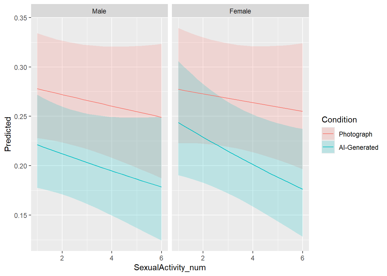

Believed

m <- glmmTMB::glmmTMB(Enticement ~ Sex / Relevance / Condition + (Relevance | Participant) + (1|Item),
                      data=filter(df, ConditionBelief == "True"), 
                      family=glmmTMB::ordbeta(),
                      control = glmmTMB::glmmTMBControl(parallel = 8))

results_table(m)

Fixed Effects

Parameter	Coefficient	SE	95% CI	z	p
(Intercept)	0.89	0.08	(0.73, 1.04)	11.25	< .001
Sex (Female)	-0.95	0.12	(-1.18, -0.73)	-8.25	< .001
Sex (Male) × RelevanceIrrelevant	-2.26	0.12	(-2.50, -2.02)	-18.45	< .001
Sex (Female) × RelevanceIrrelevant	0.04	0.13	(-0.22, 0.31)	0.33	0.738
Sex (Male) × RelevanceNon-erotic	-2.45	0.12	(-2.69, -2.22)	-20.62	< .001
Sex (Female) × RelevanceNon-erotic	-1.20	0.13	(-1.45, -0.94)	-9.16	< .001
Sex (Male) × RelevanceRelevant × ConditionAI-Generated	-0.41	0.04	(-0.48, -0.34)	-11.63	< .001
Sex (Female) × RelevanceRelevant × ConditionAI-Generated	-0.31	0.04	(-0.39, -0.22)	-7.21	< .001
Sex (Male) × RelevanceIrrelevant × ConditionAI-Generated	-0.11	0.04	(-0.18, -0.03)	-2.88	0.004
Sex (Female) × RelevanceIrrelevant × ConditionAI-Generated	-0.27	0.04	(-0.36, -0.19)	-6.16	< .001
Sex (Male) × RelevanceNon-erotic × ConditionAI-Generated	-0.23	0.05	(-0.33, -0.13)	-4.57	< .001
Sex (Female) × RelevanceNon-erotic × ConditionAI-Generated	-0.13	0.07	(-0.27, 1.90e-03)	-1.93	0.053

moderator_believed <- data.frame()
for(m in c("BAIT_Visual", "BAIT_Text", "AI_Knowledge",
           "GAAIS_Positive", "GAAIS_Negative",
           "Porn", "PornFrequency", "SexualActivity_num", 
           "Feedback_CouldDiscriminate", "Feedback_CouldNotDiscriminate",
           "Feedback_AIMoreArousing", "Feedback_AILessArousing", 
           "Feedback_LabelsIncorrect", "Feedback_LabelsReversed")) {
  moderator_believed <- rbind(moderator_believed,
                             test_moderator(filter(df, ConditionBelief == "True"), "Enticement", m))
}

display(filter(moderator_believed, p < .1))

Parameter	Coefficient	95% CI	z	p	Moderator	Outcome
Sex [Male] × ConditionAI-Generated × BAIT Text	0.31	[-0.02, 0.64]	1.84	0.066	BAIT_Text	Enticement
Sex [Female] × ConditionAI-Generated × Porn	-0.13	[-0.27, 0.01]	-1.82	0.069	Porn	Enticement
Sex [Female] × ConditionAI-Generated × SexualActivity num	-0.08	[-0.15, 0.00]	-2.01	0.045	SexualActivity_num	Enticement
Sex [Male] × ConditionAI-Generated × Feedback AILessArousingTrue	-0.32	[-0.53, -0.10]	-2.92	0.003	Feedback_AILessArousing	Enticement

Valence

valence_desc <- plot_descriptive(df, "Valence")
valence_desc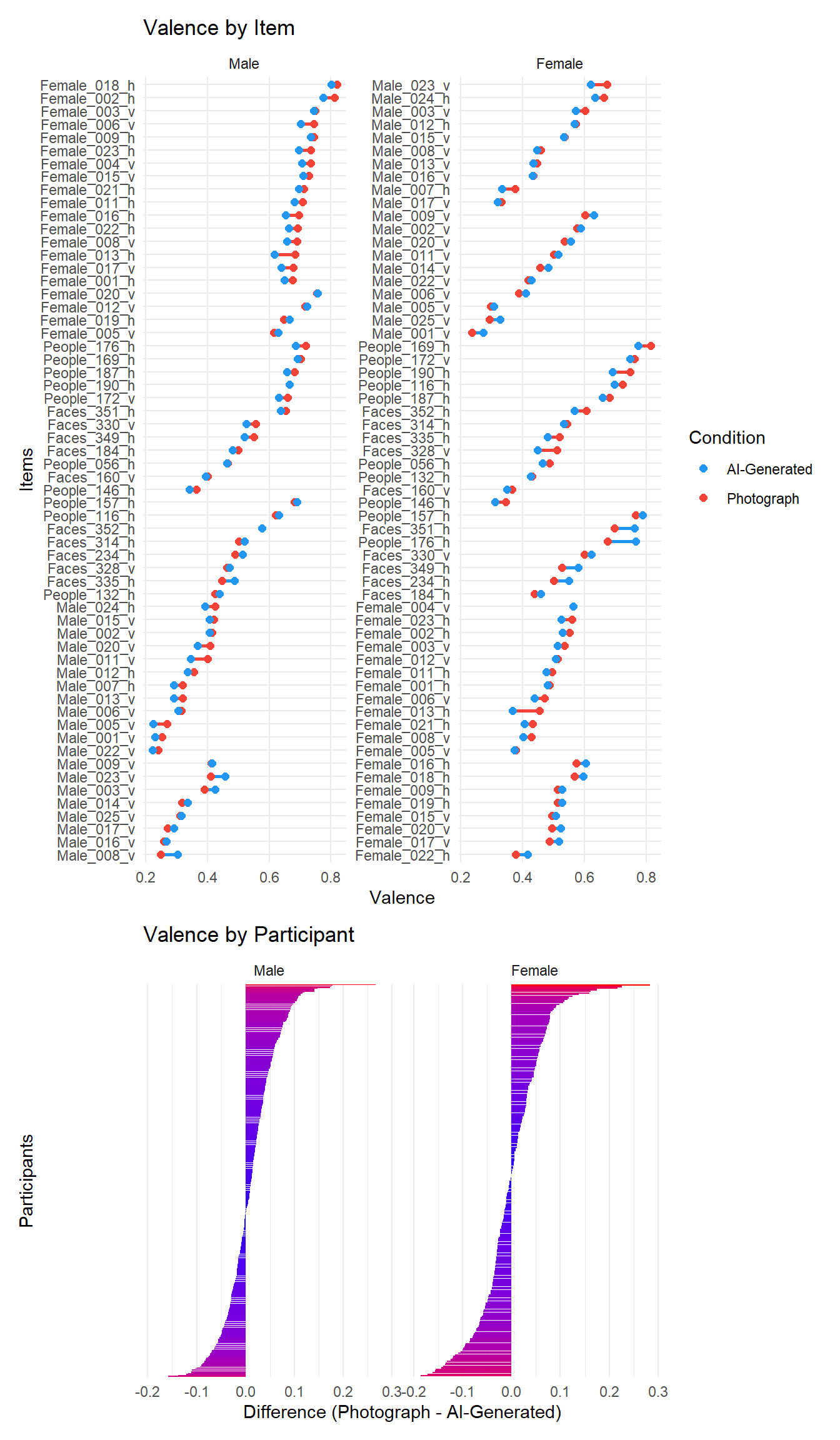

Whole Sample

This model investigates the effects of Sex, Relevance, and Condition on Valence, accounting for random variability due to participants and items (i.e., random effects).

Females rate relevant images significantly lower in valence than males on average. Males rate irrelevant and non-erotic images significantly lower in valence compared to relevant images. Females rate both irrelevant and non-erotic images higher in valence compared to relevant ones, but this effect is only significant for non-erotic stimuli. Males rate relevant images significantly lower in valence when labeled as AI-generated compared to when labeled as photographs.

Females rate relevant (photograph) images significantly lower in valence compared to males. Males rate irrelevant (photograph) and non-erotic (photograph) images significantly lower in valence compared to relevant images. Females rate non-erotic (photograph) images higher in valence compared to relevant ones. Males rate relevant AI-Generated images significantly lower in valence compared to photographs.

Lastly, we can see that for males, valence ratings are on average significantly lower for AI-Generated images compared to Photograph images. For females, there is no significant effect.

m_valence <- glmmTMB::glmmTMB(Valence ~ Sex / Relevance / Condition + 
                                (Relevance | Participant) + (1|Item),
                      data=df, family=glmmTMB::ordbeta(),
                      control = glmmTMB::glmmTMBControl(parallel = 8))

results_table(m_valence)

Fixed Effects

Parameter	Coefficient	SE	95% CI	z	p
(Intercept)	0.90	0.09	(0.73, 1.07)	10.38	< .001
Sex (Female)	-1.02	0.13	(-1.26, -0.77)	-8.07	< .001
Sex (Male) × RelevanceIrrelevant	-1.69	0.12	(-1.93, -1.45)	-13.54	< .001
Sex (Female) × RelevanceIrrelevant	0.05	0.13	(-0.21, 0.31)	0.39	0.697
Sex (Male) × RelevanceNon-erotic	-0.69	0.12	(-0.92, -0.45)	-5.72	< .001
Sex (Female) × RelevanceNon-erotic	0.49	0.13	(0.25, 0.74)	3.93	< .001
Sex (Male) × RelevanceRelevant × ConditionAI-Generated	-0.09	0.02	(-0.13, -0.06)	-5.25	< .001
Sex (Female) × RelevanceRelevant × ConditionAI-Generated	0.02	0.02	(-0.03, 0.06)	0.84	0.403
Sex (Male) × RelevanceIrrelevant × ConditionAI-Generated	-0.03	0.02	(-0.06, 8.34e-03)	-1.50	0.133
Sex (Female) × RelevanceIrrelevant × ConditionAI-Generated	-0.01	0.02	(-0.06, 0.03)	-0.49	0.621
Sex (Male) × RelevanceNon-erotic × ConditionAI-Generated	-0.03	0.02	(-0.07, 4.89e-04)	-1.93	0.053
Sex (Female) × RelevanceNon-erotic × ConditionAI-Generated	-0.02	0.02	(-0.07, 0.03)	-0.79	0.430

marginaleffects::avg_slopes(m_valence, variables="Condition", by="Sex", re.form=NA) |> 
  results_table()

Comparison	Sex	Coefficient	z	p	95% CI	predicted_lo	predicted_hi
mean(AI-Generated) - mean(Photograph)	Male	-0.01	-4.87	< .001	[-0.02, -0.01]	0.55	0.54
mean(AI-Generated) - mean(Photograph)	Female	-8.51e-04	-0.26	0.797	[-0.01, 0.01]	0.47	0.48

Subsamples

Sample

Examining the effect of sample type as a predictor, males consistently rate relevant AI-generated images significantly lower in valence compared to relevant photographs. Additionally, among non-incentivized students, this pattern persists for males, while females rate relevant AI-generated images significantly higher in valence compared to relevant photographs

m <- glmmTMB::glmmTMB(Valence ~ Sample / Sex / Relevance / Condition + (Relevance | Participant) + (1|Item),
                      data=df, 
                      family=glmmTMB::ordbeta(),
                      control = glmmTMB::glmmTMBControl(parallel = 8))

results_table(m, filter="Condition")

Fixed Effects

Parameter	Coefficient	SE	95% CI	z	p
Sample (General Population) × SexMale × RelevanceRelevant × ConditionAI-Generated	-0.11	0.02	(-0.15, -0.08)	-5.74	< .001
Sample (Students (Incentivized)) × SexMale × RelevanceRelevant × ConditionAI-Generated	-0.02	0.06	(-0.13, 0.09)	-0.36	0.719
Sample (Students (Non-incentivized)) × SexMale × RelevanceRelevant × ConditionAI-Generated	2.99e-03	0.06	(-0.11, 0.12)	0.05	0.959
Sample (General Population) × SexFemale × RelevanceRelevant × ConditionAI-Generated	0.03	0.04	(-0.05, 0.12)	0.76	0.448
Sample (Students (Incentivized)) × SexFemale × RelevanceRelevant × ConditionAI-Generated	-0.05	0.04	(-0.12, 0.02)	-1.36	0.175
Sample (Students (Non-incentivized)) × SexFemale × RelevanceRelevant × ConditionAI-Generated	0.09	0.04	(9.63e-03, 0.16)	2.21	0.027
Sample (General Population) × SexMale × RelevanceIrrelevant × ConditionAI-Generated	-0.03	0.02	(-0.07, 0.01)	-1.34	0.181
Sample (Students (Incentivized)) × SexMale × RelevanceIrrelevant × ConditionAI-Generated	-0.16	0.07	(-0.29, -0.03)	-2.36	0.018
Sample (Students (Non-incentivized)) × SexMale × RelevanceIrrelevant × ConditionAI-Generated	0.08	0.06	(-0.04, 0.19)	1.24	0.216
Sample (General Population) × SexFemale × RelevanceIrrelevant × ConditionAI-Generated	-0.02	0.04	(-0.11, 0.06)	-0.55	0.585
Sample (Students (Incentivized)) × SexFemale × RelevanceIrrelevant × ConditionAI-Generated	-0.02	0.04	(-0.09, 0.05)	-0.58	0.564
Sample (Students (Non-incentivized)) × SexFemale × RelevanceIrrelevant × ConditionAI-Generated	9.85e-03	0.04	(-0.07, 0.09)	0.25	0.802
Sample (General Population) × SexMale × RelevanceNon-erotic × ConditionAI-Generated	-0.02	0.02	(-0.06, 0.01)	-1.23	0.218
Sample (Students (Incentivized)) × SexMale × RelevanceNon-erotic × ConditionAI-Generated	-0.03	0.06	(-0.14, 0.09)	-0.46	0.644
Sample (Students (Non-incentivized)) × SexMale × RelevanceNon-erotic × ConditionAI-Generated	-0.12	0.06	(-0.24, -0.01)	-2.19	0.028
Sample (General Population) × SexFemale × RelevanceNon-erotic × ConditionAI-Generated	-0.05	0.05	(-0.14, 0.04)	-1.08	0.280
Sample (Students (Incentivized)) × SexFemale × RelevanceNon-erotic × ConditionAI-Generated	7.45e-03	0.04	(-0.07, 0.08)	0.20	0.841
Sample (Students (Non-incentivized)) × SexFemale × RelevanceNon-erotic × ConditionAI-Generated	-0.03	0.04	(-0.11, 0.06)	-0.61	0.545

Mobile

When examining the use of mobile devices as a predictor, men consistently rated the valence lower for relevant AI-generated images compared to photographs, regardless of whether they used a mobile or a standard computer. However, the effect was more pronounced among those using mobile devices.

m <- glmmTMB::glmmTMB(Valence ~ Mobile / Sex / Relevance / Condition + (Relevance | Participant) + (1|Item),
                      data=df, 
                      family=glmmTMB::ordbeta(),
                      control = glmmTMB::glmmTMBControl(parallel = 8))

results_table(m, filter="Condition")

Fixed Effects

Parameter	Coefficient	SE	95% CI	z	p
Mobile (False) × SexMale × RelevanceRelevant × ConditionAI-Generated	-0.07	0.02	(-0.11, -0.02)	-2.95	0.003
Mobile (True) × SexMale × RelevanceRelevant × ConditionAI-Generated	-0.14	0.03	(-0.20, -0.08)	-4.77	< .001
Mobile (False) × SexFemale × RelevanceRelevant × ConditionAI-Generated	9.57e-03	0.03	(-0.04, 0.06)	0.36	0.717
Mobile (True) × SexFemale × RelevanceRelevant × ConditionAI-Generated	0.05	0.05	(-0.04, 0.14)	1.06	0.290
Mobile (False) × SexMale × RelevanceIrrelevant × ConditionAI-Generated	-0.04	0.02	(-0.09, 1.15e-04)	-1.95	0.051
Mobile (True) × SexMale × RelevanceIrrelevant × ConditionAI-Generated	2.03e-03	0.03	(-0.06, 0.06)	0.07	0.945
Mobile (False) × SexFemale × RelevanceIrrelevant × ConditionAI-Generated	-0.02	0.03	(-0.07, 0.03)	-0.65	0.517
Mobile (True) × SexFemale × RelevanceIrrelevant × ConditionAI-Generated	6.72e-03	0.05	(-0.09, 0.10)	0.14	0.886
Mobile (False) × SexMale × RelevanceNon-erotic × ConditionAI-Generated	-0.02	0.02	(-0.06, 0.02)	-0.99	0.322
Mobile (True) × SexMale × RelevanceNon-erotic × ConditionAI-Generated	-0.05	0.03	(-0.11, 2.68e-03)	-1.87	0.062
Mobile (False) × SexFemale × RelevanceNon-erotic × ConditionAI-Generated	-0.01	0.03	(-0.07, 0.04)	-0.54	0.592
Mobile (True) × SexFemale × RelevanceNon-erotic × ConditionAI-Generated	-0.03	0.05	(-0.13, 0.06)	-0.66	0.507

Moderators

Here we look at whether the relationship between sex, condition and relevance and valence is moderated by AI-attitudes, porn frequency and usage, and sexual activity. Females who have more positive attitudes towards AI rated AI-generated images significantly higher in valence compared to images labelled as photographs.

Looking at feedback as a moderator we can see that ales who reported that they could not discriminate between AI-generated and photograph images, rated AI-generated images significantly higher in valence compared to images labelled as photographs.

for(m in c("BAIT_Visual", "BAIT_Text", "AI_Knowledge",
           "GAAIS_Positive", "GAAIS_Negative",
           "Porn", "PornFrequency", "SexualActivity_num")) {
  moderator_results <- rbind(moderator_results,
                             test_moderator(df, "Valence", m))
}

display(filter(moderator_results, Outcome == "Valence"))

Parameter	Coefficient	95% CI	z	p	Moderator	Outcome
Sex [Male] × ConditionAI-Generated × BAIT Visual	0.06	[-0.18, 0.31]	0.51	0.607	BAIT_Visual	Valence
Sex [Female] × ConditionAI-Generated × BAIT Visual	0.27	[-0.10, 0.64]	1.44	0.149	BAIT_Visual	Valence
Sex [Male] × ConditionAI-Generated × BAIT Text	0.10	[-0.07, 0.26]	1.13	0.259	BAIT_Text	Valence
Sex [Female] × ConditionAI-Generated × BAIT Text	0.21	[-0.04, 0.46]	1.66	0.096	BAIT_Text	Valence
Sex [Male] × ConditionAI-Generated × AI Knowledge	5.57e-03	[-0.03, 0.04]	0.31	0.755	AI_Knowledge	Valence
Sex [Female] × ConditionAI-Generated × AI Knowledge	0.04	[ 0.00, 0.08]	1.90	0.058	AI_Knowledge	Valence
Sex [Male] × ConditionAI-Generated × GAAIS Positive	0.02	[-0.17, 0.21]	0.21	0.837	GAAIS_Positive	Valence
Sex [Female] × ConditionAI-Generated × GAAIS Positive	0.36	[ 0.09, 0.63]	2.58	0.010	GAAIS_Positive	Valence
Sex [Male] × ConditionAI-Generated × GAAIS Negative	-7.48e-03	[-0.18, 0.17]	-0.08	0.932	GAAIS_Negative	Valence
Sex [Female] × ConditionAI-Generated × GAAIS Negative	0.19	[-0.07, 0.45]	1.45	0.147	GAAIS_Negative	Valence
Sex [Male] × ConditionAI-Generated × Porn	-0.04	[-0.10, 0.02]	-1.40	0.161	Porn	Valence
Sex [Female] × ConditionAI-Generated × Porn	-0.06	[-0.13, 0.01]	-1.68	0.094	Porn	Valence
Sex [Male] × ConditionAI-Generated × PornFrequency	-0.01	[-0.04, 0.01]	-0.92	0.355	PornFrequency	Valence
Sex [Female] × ConditionAI-Generated × PornFrequency	-0.01	[-0.05, 0.03]	-0.62	0.532	PornFrequency	Valence
Sex [Male] × ConditionAI-Generated × SexualActivity num	-0.02	[-0.06, 0.02]	-1.02	0.306	SexualActivity_num	Valence
Sex [Female] × ConditionAI-Generated × SexualActivity num	-0.02	[-0.06, 0.02]	-0.96	0.336	SexualActivity_num	Valence

for(m in c("Feedback_CouldDiscriminate", "Feedback_CouldNotDiscriminate",
           "Feedback_AIMoreArousing", "Feedback_AILessArousing", 
           "Feedback_LabelsIncorrect", "Feedback_LabelsReversed")) {
  feedback_results <- rbind(feedback_results,
                            test_moderator(df, "Valence", m))
}
display(filter(feedback_results, Outcome == "Valence"))

Parameter	Coefficient	95% CI	z	p	Moderator	Outcome
Sex [Male] × ConditionAI-Generated × Feedback CouldDiscriminateTrue	-0.14	[-0.29, 0.02]	-1.72	0.085	Feedback_CouldDiscriminate	Valence
Sex [Female] × ConditionAI-Generated × Feedback CouldDiscriminateTrue	-0.05	[-0.25, 0.16]	-0.45	0.653	Feedback_CouldDiscriminate	Valence
Sex [Male] × ConditionAI-Generated × Feedback CouldNotDiscriminateTrue	0.11	[ 0.03, 0.20]	2.69	0.007	Feedback_CouldNotDiscriminate	Valence
Sex [Female] × ConditionAI-Generated × Feedback CouldNotDiscriminateTrue	0.04	[-0.06, 0.14]	0.74	0.457	Feedback_CouldNotDiscriminate	Valence
Sex [Male] × ConditionAI-Generated × Feedback AIMoreArousingTrue	0.04	[-0.10, 0.18]	0.52	0.601	Feedback_AIMoreArousing	Valence
Sex [Female] × ConditionAI-Generated × Feedback AIMoreArousingTrue	0.13	[-0.02, 0.27]	1.71	0.088	Feedback_AIMoreArousing	Valence
Sex [Male] × ConditionAI-Generated × Feedback AILessArousingTrue	-0.10	[-0.23, 0.03]	-1.49	0.137	Feedback_AILessArousing	Valence
Sex [Female] × ConditionAI-Generated × Feedback AILessArousingTrue	0.07	[-0.11, 0.25]	0.77	0.442	Feedback_AILessArousing	Valence
Sex [Male] × ConditionAI-Generated × Feedback LabelsIncorrectTrue	-0.05	[-0.14, 0.03]	-1.34	0.181	Feedback_LabelsIncorrect	Valence
Sex [Female] × ConditionAI-Generated × Feedback LabelsIncorrectTrue	-0.08	[-0.19, 0.03]	-1.40	0.161	Feedback_LabelsIncorrect	Valence
Sex [Male] × ConditionAI-Generated × Feedback LabelsReversedTrue	-5.72e-03	[-0.19, 0.18]	-0.06	0.952	Feedback_LabelsReversed	Valence
Sex [Female] × ConditionAI-Generated × Feedback LabelsReversedTrue	0.08	[-0.12, 0.28]	0.80	0.426	Feedback_LabelsReversed	Valence

Believed

m <- glmmTMB::glmmTMB(Valence ~ Sex / Relevance / Condition + (Relevance | Participant) + (1|Item),
                      data=filter(df, ConditionBelief == "True"), 
                      family=glmmTMB::ordbeta(),
                      control = glmmTMB::glmmTMBControl(parallel = 8))

results_table(m)

Fixed Effects

Parameter	Coefficient	SE	95% CI	z	p
(Intercept)	0.95	0.09	(0.78, 1.12)	11.07	< .001
Sex (Female)	-0.95	0.13	(-1.19, -0.70)	-7.56	< .001
Sex (Male) × RelevanceIrrelevant	-1.68	0.12	(-1.92, -1.44)	-13.59	< .001
Sex (Female) × RelevanceIrrelevant	0.03	0.13	(-0.23, 0.28)	0.20	0.839
Sex (Male) × RelevanceNon-erotic	-0.72	0.12	(-0.95, -0.48)	-6.02	< .001
Sex (Female) × RelevanceNon-erotic	0.42	0.12	(0.18, 0.67)	3.39	< .001
Sex (Male) × RelevanceRelevant × ConditionAI-Generated	-0.48	0.03	(-0.54, -0.41)	-14.51	< .001
Sex (Female) × RelevanceRelevant × ConditionAI-Generated	-0.33	0.04	(-0.41, -0.26)	-8.44	< .001
Sex (Male) × RelevanceIrrelevant × ConditionAI-Generated	-0.20	0.03	(-0.27, -0.14)	-6.30	< .001
Sex (Female) × RelevanceIrrelevant × ConditionAI-Generated	-0.24	0.04	(-0.31, -0.16)	-5.92	< .001
Sex (Male) × RelevanceNon-erotic × ConditionAI-Generated	-0.17	0.04	(-0.24, -0.10)	-4.76	< .001
Sex (Female) × RelevanceNon-erotic × ConditionAI-Generated	-0.22	0.06	(-0.32, -0.11)	-3.91	< .001

moderator_believed <- data.frame()
for(m in c("BAIT_Visual", "BAIT_Text", "AI_Knowledge",
           "GAAIS_Positive", "GAAIS_Negative",
           "Porn", "PornFrequency", "SexualActivity_num", 
           "Feedback_CouldDiscriminate", "Feedback_CouldNotDiscriminate",
           "Feedback_AIMoreArousing", "Feedback_AILessArousing", 
           "Feedback_LabelsIncorrect", "Feedback_LabelsReversed")) {
  moderator_believed <- rbind(moderator_believed,
                             test_moderator(filter(df, ConditionBelief == "True"), "Valence", m))
}

display(filter(moderator_believed, p < .1))

Parameter	Coefficient	95% CI	z	p	Moderator	Outcome
Sex [Male] × ConditionAI-Generated × BAIT Text	0.38	[ 0.02, 0.74]	2.06	0.040	BAIT_Text	Valence
Sex [Male] × ConditionAI-Generated × Feedback CouldDiscriminateTrue	-0.30	[-0.62, 0.02]	-1.81	0.071	Feedback_CouldDiscriminate	Valence
Sex [Female] × ConditionAI-Generated × Feedback CouldNotDiscriminateTrue	0.20	[-0.02, 0.41]	1.82	0.069	Feedback_CouldNotDiscriminate	Valence
Sex [Male] × ConditionAI-Generated × Feedback AILessArousingTrue	-0.21	[-0.45, 0.03]	-1.70	0.090	Feedback_AILessArousing	Valence

Emotionality (Combined Factor)

Here we combined the data for arousal, valence and enticing into an emotionality factor.

pca <- principal_components(df[c("Valence", "Arousal", "Enticement")], n = 2)
pca

# Loadings from Principal Component Analysis (no rotation)

Variable   | PC1  |  PC2  | Complexity
--------------------------------------
Valence    | 0.79 | 0.61  |    1.87   
Arousal    | 0.87 | -0.37 |    1.34   
Enticement | 0.91 | -0.17 |    1.07   

The 2 principal components accounted for 91.56% of the total variance of the original data (PC1 = 73.77%, PC2 = 17.79%).

df$Emotionality <- normalize(predict(pca)$PC1)

emotionality <- df |> 
  mutate(Emotionality_Extreme = ifelse(Emotionality %in% c(0, 1), "Extreme", "Not extreme")) |>
  ggplot(aes(x=Emotionality, fill=Relevance)) +
  geom_histogram(aes(color=Emotionality_Extreme), position = "identity", bins=80) +
  facet_grid(Relevance~Sex, scales="free_y") +
  scale_color_manual(values=c("red", "white"), guide="none") +
  scale_fill_manual(values=c("Relevant"="#E91E63", "Irrelevant"="#FF9800", "Non-erotic"="#03A9F4"), guide="none") +
  scale_y_sqrt(expand = c(0, 0)) +
  labs(title = "Emotionality") +
  theme_abyss() +
  theme(plot.title = element_text(hjust = 0.5, face="bold"))

emotionality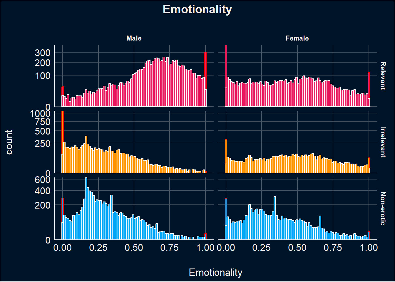

emotionality_desc <- plot_descriptive(df, "Emotionality")
emotionality_desc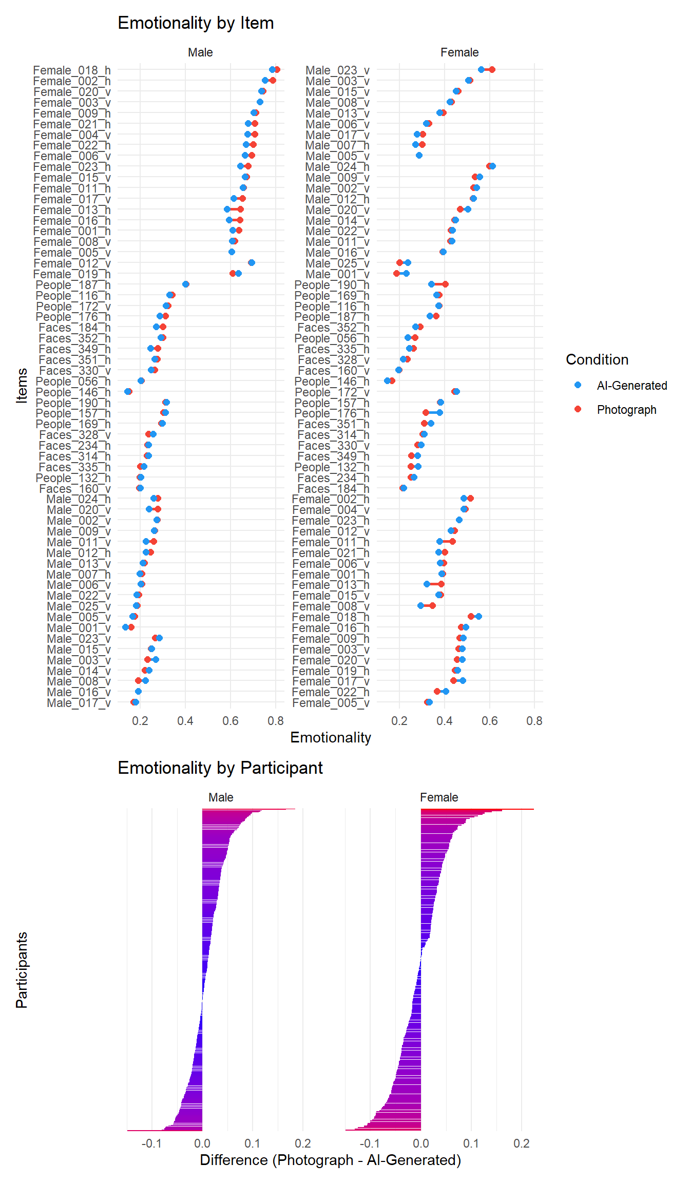

Whole Sample

This model looks at the effect of sex, relevance and condition on emotionality, accounting for random variability due to participants and items (i.e., random effects).

These findings suggest that females consistently rate relevant (photograph) images lower in emotionality compared to males. Additionally, males specifically rate irrelevant (photograph) images lower in emotionality, and both genders rate non-erotic (photgraph) images lower in emotionality compared to relevant images. Furthermore, males rate AI-generated relevant images lower in emotionality compared to those labelled as photographs.

For males, emotionality ratings are on average significantly lower for AI-Generated images compared to Photograph images. This indicates that males generally rate AI-Generated images lower in emotionality compared to photographs. For females, there is no significant difference between the mean ratings of AI-Generated and Photograph images in terms of emotionality. This suggests that females do not show a significant preference or difference in emotionality ratings between AI-Generated and Photograph images.

m <- glmmTMB::glmmTMB(Emotionality ~ Sex / Relevance / Condition + (Relevance | Participant) + (1|Item),
                      data=df, family=glmmTMB::ordbeta(),
                      control = glmmTMB::glmmTMBControl(parallel = 8))

results_table(m)

Fixed Effects

Parameter	Coefficient	SE	95% CI	z	p
(Intercept)	0.81	0.08	(0.66, 0.96)	10.67	< .001
Sex (Female)	-1.23	0.11	(-1.45, -1.01)	-10.96	< .001
Sex (Male) × RelevanceIrrelevant	-2.28	0.11	(-2.49, -2.06)	-20.73	< .001
Sex (Female) × RelevanceIrrelevant	0.02	0.12	(-0.21, 0.26)	0.18	0.861
Sex (Male) × RelevanceNon-erotic	-1.80	0.10	(-2.00, -1.60)	-17.65	< .001
Sex (Female) × RelevanceNon-erotic	-0.47	0.11	(-0.68, -0.26)	-4.38	< .001
Sex (Male) × RelevanceRelevant × ConditionAI-Generated	-0.09	0.02	(-0.12, -0.06)	-6.10	< .001
Sex (Female) × RelevanceRelevant × ConditionAI-Generated	0.02	0.02	(-0.02, 0.06)	1.11	0.267
Sex (Male) × RelevanceIrrelevant × ConditionAI-Generated	-0.02	0.02	(-0.05, 0.02)	-1.03	0.305
Sex (Female) × RelevanceIrrelevant × ConditionAI-Generated	-8.79e-05	0.02	(-0.04, 0.04)	-4.33e-03	0.997
Sex (Male) × RelevanceNon-erotic × ConditionAI-Generated	-0.02	0.02	(-0.05, 7.10e-03)	-1.50	0.132
Sex (Female) × RelevanceNon-erotic × ConditionAI-Generated	5.19e-03	0.02	(-0.03, 0.04)	0.26	0.798

marginaleffects::avg_slopes(m, variables="Condition", by="Sex", re.form=NA) |> 
  results_table()

Comparison	Sex	Coefficient	z	p	95% CI	predicted_lo	predicted_hi
mean(AI-Generated) - mean(Photograph)	Male	-9.25e-03	-5.27	< .001	[-0.01, -0.01]	0.27	0.27
mean(AI-Generated) - mean(Photograph)	Female	2.16e-03	0.80	0.423	[ 0.00, 0.01]	0.40	0.40

Subsamples

Sample

This model investigates the influence of sample type (General Population, Incentivized Students, Non-incentivized Students), Sex, Relevance, and Condition (AI-Generated vs. Photograph) on emotionality ratings. Males from the General Population consistently rated AI-Generated images lower in emotionality compared to photographs across relevant conditions. Females from the Non-incentivized Students group showed a significant preference for AI-Generated images in terms of emotionality compared to photographs.

These findings suggest that the perception of emotionality in AI-Generated images varies significantly based on sample type (general population vs. students) and the relevance of the images, particularly for males and non-incentivized female students.

m <- glmmTMB::glmmTMB(Emotionality ~ Sample / Sex / Relevance / Condition + (Relevance | Participant) + (1|Item),
                      data=df, 
                      family=glmmTMB::ordbeta(),
                      control = glmmTMB::glmmTMBControl(parallel = 8))

results_table(m, filter="Condition")

Fixed Effects

Parameter	Coefficient	SE	95% CI	z	p
Sample (General Population) × SexMale × RelevanceRelevant × ConditionAI-Generated	-0.11	0.02	(-0.14, -0.07)	-6.17	< .001
Sample (Students (Incentivized)) × SexMale × RelevanceRelevant × ConditionAI-Generated	-0.09	0.05	(-0.19, 5.84e-03)	-1.85	0.065
Sample (Students (Non-incentivized)) × SexMale × RelevanceRelevant × ConditionAI-Generated	-3.69e-03	0.05	(-0.10, 0.09)	-0.08	0.938
Sample (General Population) × SexFemale × RelevanceRelevant × ConditionAI-Generated	0.01	0.04	(-0.06, 0.09)	0.30	0.764
Sample (Students (Incentivized)) × SexFemale × RelevanceRelevant × ConditionAI-Generated	-0.04	0.03	(-0.10, 0.03)	-1.06	0.288
Sample (Students (Non-incentivized)) × SexFemale × RelevanceRelevant × ConditionAI-Generated	0.09	0.03	(0.03, 0.16)	2.74	0.006
Sample (General Population) × SexMale × RelevanceIrrelevant × ConditionAI-Generated	-0.02	0.02	(-0.05, 0.02)	-0.87	0.383
Sample (Students (Incentivized)) × SexMale × RelevanceIrrelevant × ConditionAI-Generated	-0.12	0.06	(-0.24, 8.06e-03)	-1.83	0.067
Sample (Students (Non-incentivized)) × SexMale × RelevanceIrrelevant × ConditionAI-Generated	0.05	0.06	(-0.06, 0.16)	0.88	0.381
Sample (General Population) × SexFemale × RelevanceIrrelevant × ConditionAI-Generated	0.01	0.04	(-0.06, 0.09)	0.34	0.735
Sample (Students (Incentivized)) × SexFemale × RelevanceIrrelevant × ConditionAI-Generated	-0.03	0.03	(-0.09, 0.04)	-0.78	0.435
Sample (Students (Non-incentivized)) × SexFemale × RelevanceIrrelevant × ConditionAI-Generated	0.02	0.03	(-0.05, 0.09)	0.51	0.607
Sample (General Population) × SexMale × RelevanceNon-erotic × ConditionAI-Generated	-0.02	0.02	(-0.05, 0.01)	-1.15	0.249
Sample (Students (Incentivized)) × SexMale × RelevanceNon-erotic × ConditionAI-Generated	3.58e-03	0.05	(-0.10, 0.11)	0.07	0.945
Sample (Students (Non-incentivized)) × SexMale × RelevanceNon-erotic × ConditionAI-Generated	-0.07	0.05	(-0.16, 0.02)	-1.50	0.133
Sample (General Population) × SexFemale × RelevanceNon-erotic × ConditionAI-Generated	2.43e-03	0.04	(-0.07, 0.08)	0.06	0.950
Sample (Students (Incentivized)) × SexFemale × RelevanceNon-erotic × ConditionAI-Generated	7.96e-03	0.03	(-0.06, 0.07)	0.24	0.813
Sample (Students (Non-incentivized)) × SexFemale × RelevanceNon-erotic × ConditionAI-Generated	4.41e-03	0.03	(-0.06, 0.07)	0.13	0.895

Mobile

This analysis explores the influence of using a mobile device to complete the experiment on emotionality ratings, focusing on differences between males and females across relevant and irrelevant conditions of AI-Generated and photograph images.

Males consistently rate emotionality significantly lower for relevant AI-Generated images compared to photograph images, irrespective of whether they use a mobile device or not. They also rate emotionality significantly lower for irrelevant AI-Generated images compared to photograph images when not using a mobile device. For females, there are no significant differences in how they rate emotionality for AI-Generated images based on whether they use a mobile device or not, regardless of relevance.

These findings highlight that the perception of emotionality in AI-Generated images among males is notably affected by the use of mobile devices during the experiment, whereas females show no significant variation in their ratings based on device usage.

m <- glmmTMB::glmmTMB(Emotionality ~ Mobile / Sex / Relevance / Condition + (Relevance | Participant) + (1|Item),
                      data=df, 
                      family=glmmTMB::ordbeta(),
                      control = glmmTMB::glmmTMBControl(parallel = 8))

results_table(m, filter="Condition")

Fixed Effects

Parameter	Coefficient	SE	95% CI	z	p
Mobile (False) × SexMale × RelevanceRelevant × ConditionAI-Generated	-0.07	0.02	(-0.11, -0.03)	-3.75	< .001
Mobile (True) × SexMale × RelevanceRelevant × ConditionAI-Generated	-0.13	0.03	(-0.18, -0.08)	-5.15	< .001
Mobile (False) × SexFemale × RelevanceRelevant × ConditionAI-Generated	0.03	0.02	(-0.02, 0.07)	1.19	0.234
Mobile (True) × SexFemale × RelevanceRelevant × ConditionAI-Generated	6.59e-03	0.04	(-0.07, 0.09)	0.16	0.873
Mobile (False) × SexMale × RelevanceIrrelevant × ConditionAI-Generated	-0.05	0.02	(-0.10, -0.01)	-2.47	0.013
Mobile (True) × SexMale × RelevanceIrrelevant × ConditionAI-Generated	0.04	0.03	(-0.01, 0.10)	1.50	0.135
Mobile (False) × SexFemale × RelevanceIrrelevant × ConditionAI-Generated	-0.01	0.02	(-0.06, 0.03)	-0.51	0.610
Mobile (True) × SexFemale × RelevanceIrrelevant × ConditionAI-Generated	0.04	0.04	(-0.04, 0.12)	0.90	0.370
Mobile (False) × SexMale × RelevanceNon-erotic × ConditionAI-Generated	-0.02	0.02	(-0.05, 0.02)	-0.81	0.416
Mobile (True) × SexMale × RelevanceNon-erotic × ConditionAI-Generated	-0.04	0.03	(-0.09, 0.01)	-1.41	0.157
Mobile (False) × SexFemale × RelevanceNon-erotic × ConditionAI-Generated	6.63e-03	0.02	(-0.04, 0.05)	0.29	0.775
Mobile (True) × SexFemale × RelevanceNon-erotic × ConditionAI-Generated	4.03e-04	0.04	(-0.08, 0.08)	9.59e-03	0.992

Moderators

Looking at AI-attitudes, porn frequency and usage, sexual activity, and feedback as moderators, the analysis showed that for females, having a positive attitude towards AI significantly increased their emotionality ratings for AI-generated images compared to those who did not have such positive attitudes. Additionally, for females reporting finding AI more arousing lowered their emotionality ratings for AI-generated images compared to those that did not. This effect was significantly reversed for males.

for(m in c("BAIT_Visual", "BAIT_Text", "AI_Knowledge",
           "GAAIS_Positive", "GAAIS_Negative",
           "Porn", "PornFrequency", "SexualActivity_num")) {
  moderator_results <- rbind(moderator_results,
                             test_moderator(df, "Emotionality", m))
}

display(filter(moderator_results, Outcome == "Emotionality"))

Parameter	Coefficient	95% CI	z	p	Moderator	Outcome
Sex [Male] × ConditionAI-Generated × BAIT Visual	0.03	[-0.20, 0.25]	0.24	0.813	BAIT_Visual	Emotionality
Sex [Female] × ConditionAI-Generated × BAIT Visual	0.26	[-0.09, 0.61]	1.47	0.141	BAIT_Visual	Emotionality
Sex [Male] × ConditionAI-Generated × BAIT Text	0.03	[-0.13, 0.18]	0.33	0.738	BAIT_Text	Emotionality
Sex [Female] × ConditionAI-Generated × BAIT Text	0.12	[-0.11, 0.35]	1.00	0.317	BAIT_Text	Emotionality
Sex [Male] × ConditionAI-Generated × AI Knowledge	9.49e-03	[-0.02, 0.04]	0.57	0.568	AI_Knowledge	Emotionality
Sex [Female] × ConditionAI-Generated × AI Knowledge	0.01	[-0.03, 0.05]	0.65	0.516	AI_Knowledge	Emotionality
Sex [Male] × ConditionAI-Generated × GAAIS Positive	0.06	[-0.12, 0.24]	0.66	0.508	GAAIS_Positive	Emotionality
Sex [Female] × ConditionAI-Generated × GAAIS Positive	0.30	[ 0.04, 0.56]	2.27	0.023	GAAIS_Positive	Emotionality
Sex [Male] × ConditionAI-Generated × GAAIS Negative	0.02	[-0.14, 0.18]	0.21	0.831	GAAIS_Negative	Emotionality
Sex [Female] × ConditionAI-Generated × GAAIS Negative	0.13	[-0.12, 0.37]	1.01	0.311	GAAIS_Negative	Emotionality
Sex [Male] × ConditionAI-Generated × Porn	-0.04	[-0.09, 0.01]	-1.54	0.123	Porn	Emotionality
Sex [Female] × ConditionAI-Generated × Porn	-0.06	[-0.13, 0.01]	-1.81	0.071	Porn	Emotionality
Sex [Male] × ConditionAI-Generated × PornFrequency	-0.01	[-0.04, 0.01]	-1.04	0.299	PornFrequency	Emotionality
Sex [Female] × ConditionAI-Generated × PornFrequency	-2.12e-03	[-0.04, 0.04]	-0.11	0.912	PornFrequency	Emotionality
Sex [Male] × ConditionAI-Generated × SexualActivity num	-0.01	[-0.05, 0.02]	-0.71	0.475	SexualActivity_num	Emotionality
Sex [Female] × ConditionAI-Generated × SexualActivity num	-0.03	[-0.07, 0.01]	-1.66	0.097	SexualActivity_num	Emotionality

For females reporting finding AI more arousing lowered their emotionality ratings for AI-generated images compared to those that did not. This effect was significantly reversed for males.

for(m in c("Feedback_CouldDiscriminate", "Feedback_CouldNotDiscriminate",
           "Feedback_AIMoreArousing", "Feedback_AILessArousing", 
           "Feedback_LabelsIncorrect", "Feedback_LabelsReversed")) {
  feedback_results <- rbind(feedback_results,
                            test_moderator(df, "Emotionality", m))
}
display(filter(feedback_results, Outcome == "Emotionality"))

Parameter	Coefficient	95% CI	z	p	Moderator	Outcome
Sex [Male] × ConditionAI-Generated × Feedback CouldDiscriminateTrue	-0.05	[-0.19, 0.09]	-0.71	0.478	Feedback_CouldDiscriminate	Emotionality
Sex [Female] × ConditionAI-Generated × Feedback CouldDiscriminateTrue	-0.16	[-0.36, 0.03]	-1.62	0.105	Feedback_CouldDiscriminate	Emotionality
Sex [Male] × ConditionAI-Generated × Feedback CouldNotDiscriminateTrue	0.05	[-0.03, 0.13]	1.28	0.200	Feedback_CouldNotDiscriminate	Emotionality
Sex [Female] × ConditionAI-Generated × Feedback CouldNotDiscriminateTrue	-5.98e-03	[-0.11, 0.09]	-0.12	0.906	Feedback_CouldNotDiscriminate	Emotionality
Sex [Male] × ConditionAI-Generated × Feedback AIMoreArousingTrue	0.04	[-0.09, 0.17]	0.55	0.580	Feedback_AIMoreArousing	Emotionality
Sex [Female] × ConditionAI-Generated × Feedback AIMoreArousingTrue	0.14	[ 0.00, 0.27]	1.96	0.050	Feedback_AIMoreArousing	Emotionality
Sex [Male] × ConditionAI-Generated × Feedback AILessArousingTrue	-0.16	[-0.28, -0.04]	-2.58	0.010	Feedback_AILessArousing	Emotionality
Sex [Female] × ConditionAI-Generated × Feedback AILessArousingTrue	0.13	[-0.04, 0.30]	1.47	0.142	Feedback_AILessArousing	Emotionality
Sex [Male] × ConditionAI-Generated × Feedback LabelsIncorrectTrue	-0.05	[-0.13, 0.02]	-1.44	0.150	Feedback_LabelsIncorrect	Emotionality
Sex [Female] × ConditionAI-Generated × Feedback LabelsIncorrectTrue	-0.06	[-0.17, 0.05]	-1.07	0.284	Feedback_LabelsIncorrect	Emotionality
Sex [Male] × ConditionAI-Generated × Feedback LabelsReversedTrue	-0.05	[-0.23, 0.12]	-0.61	0.543	Feedback_LabelsReversed	Emotionality
Sex [Female] × ConditionAI-Generated × Feedback LabelsReversedTrue	0.08	[-0.11, 0.27]	0.85	0.393	Feedback_LabelsReversed	Emotionality

Believed

m <- glmmTMB::glmmTMB(Emotionality ~ Sex / Relevance / Condition + (Relevance | Participant) + (1|Item),
                      data=filter(df, ConditionBelief == "True"), 
                      family=glmmTMB::ordbeta(),
                      control = glmmTMB::glmmTMBControl(parallel = 8))

results_table(m)

Fixed Effects

Parameter	Coefficient	SE	95% CI	z	p
(Intercept)	0.87	0.08	(0.72, 1.02)	11.46	< .001
Sex (Female)	-1.15	0.11	(-1.37, -0.93)	-10.32	< .001
Sex (Male) × RelevanceIrrelevant	-2.29	0.11	(-2.51, -2.08)	-21.03	< .001
Sex (Female) × RelevanceIrrelevant	-0.01	0.12	(-0.25, 0.22)	-0.12	0.906
Sex (Male) × RelevanceNon-erotic	-1.85	0.10	(-2.05, -1.65)	-18.13	< .001
Sex (Female) × RelevanceNon-erotic	-0.57	0.11	(-0.78, -0.36)	-5.32	< .001
Sex (Male) × RelevanceRelevant × ConditionAI-Generated	-0.47	0.03	(-0.53, -0.42)	-16.28	< .001
Sex (Female) × RelevanceRelevant × ConditionAI-Generated	-0.38	0.04	(-0.45, -0.31)	-10.80	< .001
Sex (Male) × RelevanceIrrelevant × ConditionAI-Generated	-0.15	0.03	(-0.21, -0.09)	-4.96	< .001
Sex (Female) × RelevanceIrrelevant × ConditionAI-Generated	-0.25	0.04	(-0.32, -0.18)	-7.00	< .001
Sex (Male) × RelevanceNon-erotic × ConditionAI-Generated	-0.15	0.03	(-0.22, -0.09)	-4.63	< .001
Sex (Female) × RelevanceNon-erotic × ConditionAI-Generated	-0.13	0.05	(-0.22, -0.04)	-2.76	0.006

moderator_believed <- data.frame()
for(m in c("BAIT_Visual", "BAIT_Text", "AI_Knowledge",
           "GAAIS_Positive", "GAAIS_Negative",
           "Porn", "PornFrequency", "SexualActivity_num", 
           "Feedback_CouldDiscriminate", "Feedback_CouldNotDiscriminate",
           "Feedback_AIMoreArousing", "Feedback_AILessArousing", 
           "Feedback_LabelsIncorrect", "Feedback_LabelsReversed")) {
  moderator_believed <- rbind(moderator_believed,
                             test_moderator(filter(df, ConditionBelief == "True"), "Emotionality", m))
}

display(filter(moderator_believed, p < .1))

Parameter	Coefficient	95% CI	z	p	Moderator	Outcome
Sex [Male] × ConditionAI-Generated × BAIT Text	0.32	[-0.03, 0.66]	1.77	0.076	BAIT_Text	Emotionality
Sex [Female] × ConditionAI-Generated × Porn	-0.13	[-0.27, 0.02]	-1.69	0.091	Porn	Emotionality
Sex [Female] × ConditionAI-Generated × SexualActivity num	-0.08	[-0.16, 0.00]	-1.97	0.049	SexualActivity_num	Emotionality
Sex [Female] × ConditionAI-Generated × Feedback CouldDiscriminateTrue	-0.35	[-0.74, 0.04]	-1.77	0.077	Feedback_CouldDiscriminate	Emotionality
Sex [Male] × ConditionAI-Generated × Feedback AILessArousingTrue	-0.31	[-0.54, -0.08]	-2.69	0.007	Feedback_AILessArousing	Emotionality

Summary

• Believing erotic images to be AI-generated, regardless of its true nature, leads to a less pleasurable experience (i.e., a less intense and less positive emotion). While the effect is the most noticeable for men (who experience a stronger arousal when exposed to the images), it appears overall very small in magnitude. However, it becomes more pronounced for both genders when controlled for the belief in the images’ nature, and is consistent with participants’ feedback, suggesting an important meta-cognitive component (in the form of explicitly conscious beliefs).
• The items developed (BAIT scale) seem to measure a different dimension to AI-expertise.

Figures

pred1 <- rbind(
  marginaleffects::predictions(m_arousal, by=c("Sex", "Relevance", "Condition"), newdata = "marginalmeans", re.form=NA) |>
  as.data.frame() |> 
  mutate(Outcome="Arousal"),
  marginaleffects::predictions(m_enticement, by=c("Sex", "Relevance", "Condition"), newdata = "marginalmeans", re.form=NA) |>
  as.data.frame() |> 
  mutate(Outcome="Enticement"),
  marginaleffects::predictions(m_valence, by=c("Sex", "Relevance", "Condition"), newdata = "marginalmeans", re.form=NA) |>
  as.data.frame() |> 
  mutate(Outcome="Valence")
)

stars1 <- data.frame(label=c("***", "***", "*", "***"), 
                    Sex=fct_relevel(c("Male", "Male", "Male", "Male"), "Male"), 
                    Relevance=c("Relevant", "Relevant", "Non-erotic", "Relevant"), 
                    Outcome=c("Arousal", "Enticement", "Enticement", "Valence"),
                    y=c(0.75, 0.8, 0.2, 0.8))

p1 <- pred1 |>
  mutate(Sex = fct_relevel(Sex, "Male", "Female")) |> 
  ggplot(aes(x=Relevance, y=estimate)) +
  geom_hline(yintercept=0, color="darkgrey") +
  geom_line(aes(group=Condition, color=Condition), position = position_dodge(width=0.2), alpha=0.8, linewidth=0.2) +
  geom_pointrange(aes(ymin = conf.low, ymax=conf.high, color=Condition), position = position_dodge(width=0.2), size=0.2) +
  geom_text(data=stars1, aes(y=y, label=label), hjust=0.5, size=3) +
  geom_rect(data=data.frame(Type="All trials", estimate=0.1, Sex=as.factor("Male"), Outcome="Arousal", Relevance="Relevant"), 
            aes(xmin=0.8, xmax=1.2, ymin=0.5, ymax=0.80), color="#8BC34A", alpha=0) +
  geom_rect(data=data.frame(Type="All trials", estimate=0.1, Sex=as.factor("Female"), Outcome="Arousal", Relevance="Relevant"), 
            aes(xmin=0.8, xmax=1.2, ymin=0.2, ymax=0.5), color="#8BC34A", alpha=0) +
  facet_grid(Outcome~Sex, switch="y") +
  scale_y_continuous(limits=c(0, 1), labels=scales::percent) +
  scale_color_manual(values=c("AI-Generated"="#2196F3", "Photograph"="#F44336")) +
  theme_minimal() +
  theme(axis.title.y = element_blank(),
        axis.title.x = element_blank(),
        axis.text.y = element_text(size = 8),
        strip.placement = "outside",
        strip.background.x = element_rect(fill=c("lightgrey"), color=NA),
        strip.text.x = element_text(size = 10),
        strip.text.y = element_text(size = 10),
        axis.text.x = element_text(angle=25, hjust=1, vjust=1.1, size=9, color="black"),
        legend.text = element_text(size = 10),
        legend.position = ) +
  labs(color="Images presented as:",
       tag = "A")
p1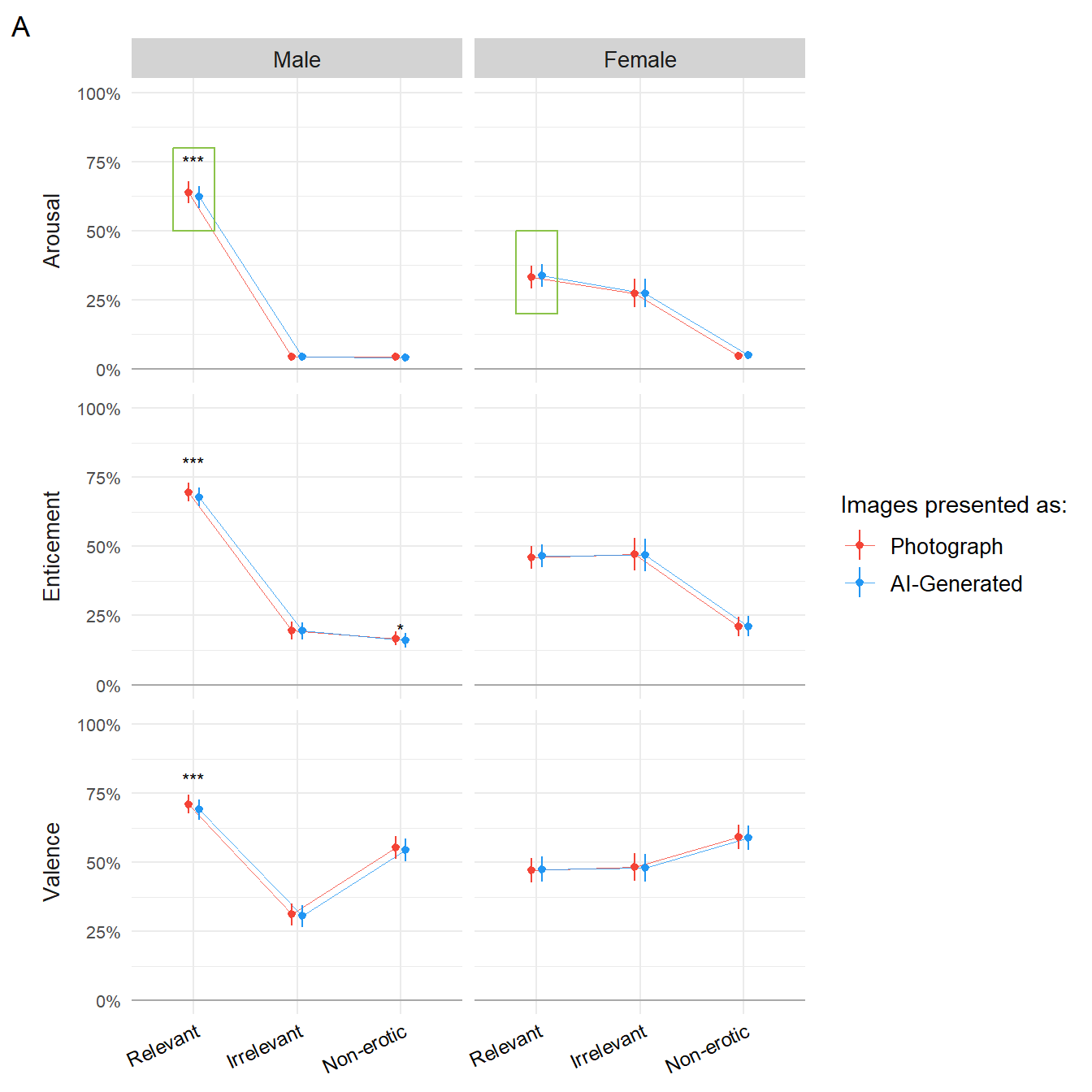

m1 <- glmmTMB::glmmTMB(Arousal ~ Sex / Condition + (Condition | Participant) + (1|Item),
                      data=filter(df, Relevance=="Relevant"), 
                      family=glmmTMB::ordbeta(),
                      control = glmmTMB::glmmTMBControl(parallel = 8))
m2 <- glmmTMB::glmmTMB(Arousal ~ Sex / Condition + (Condition | Participant) + (1|Item),
                      data=filter(df, Relevance=="Relevant", ConditionBelief == "True"), 
                      family=glmmTMB::ordbeta(),
                      control = glmmTMB::glmmTMBControl(parallel = 8))
m3 <- glmmTMB::glmmTMB(Arousal ~ Sex / Condition  + (Condition | Participant) + (1|Item),
                      data=filter(df, Relevance=="Relevant", ConditionBelief == "True", Feedback_AILessArousing=="True"), 
                      family=glmmTMB::ordbeta(),
                      control = glmmTMB::glmmTMBControl(parallel = 8))

stars2 <- data.frame(label=c("***", "***", "***", "***", "*"), 
                    Sex=fct_relevel(c("Male", "Male", "Male", "Female", "Female"), 
                                    "Male", "Female"), 
                    Type=c("All trials", "Believed trials", "'AI was less arousing'", "Believed trials", "'AI was less arousing'"), 
                    y=c(0.76, 0.76, 0.76, 0.45, 0.45))

pred2 <- rbind(
  estimate_relation(m1) |> 
    mutate(Type = "All trials"),
  estimate_relation(m2) |> 
    mutate(Type = "Believed trials"),
  estimate_relation(m3) |> 
    mutate(Type = "'AI was less arousing'")
)

p2 <- pred2 |> 
  mutate(Type = fct_relevel(Type, "All trials", "Believed trials", "'AI was less arousing'")) |> 
  ggplot(aes(x=Type, y=Predicted)) +
  geom_hline(yintercept=0, color="darkgrey") +
  geom_line(aes(group=Condition, color=Condition), position = position_dodge(width=0.2), alpha=0.8, linewidth=0.1) +
  geom_bar(stat="identity", aes(fill=Condition), position = position_dodge(width=0.2), width=0.2, alpha=0.6) +
  geom_pointrange(aes(ymin = CI_low, ymax=CI_high, color=Condition), position = position_dodge(width=0.2), size=0.2) +
  geom_rect(data=data.frame(Type="All trials", Predicted=0.1, Sex=as.factor("Male")), 
            aes(xmin=0.7, xmax=1.3, ymin=0.55, ymax=0.7), color="#8BC34A", alpha=0) +
  geom_rect(data=data.frame(Type="All trials", Predicted=0.1, Sex=as.factor("Female")), 
            aes(xmin=0.7, xmax=1.3, ymin=0.25, ymax=0.4), color="#8BC34A", alpha=0) +
  geom_text(data=stars2, aes(y=y, label=label), hjust=0.5, size=3) +
  facet_grid(~Sex) +
  scale_y_continuous(labels=scales::percent) +
  scale_color_manual(values=c("AI-Generated"="#2196F3", "Photograph"="#F44336")) +
  scale_fill_manual(values=c("AI-Generated"="#2196F3", "Photograph"="#F44336")) +
  labs(y="Arousal",
       tag = "B") +
  theme_minimal() +
  theme(axis.title.x = element_blank(),
        axis.text.x = element_text(angle=25, hjust=1, vjust=1.1, size=9),
        axis.text.y = element_text(size = 8),
        axis.title.y = element_text(size = 10),
        strip.placement = "outside",
        strip.background.x = element_rect(fill=c("lightgrey"), color=NA),
        strip.text.x = element_text(size = 10),
        legend.position = "none")


p1 | p2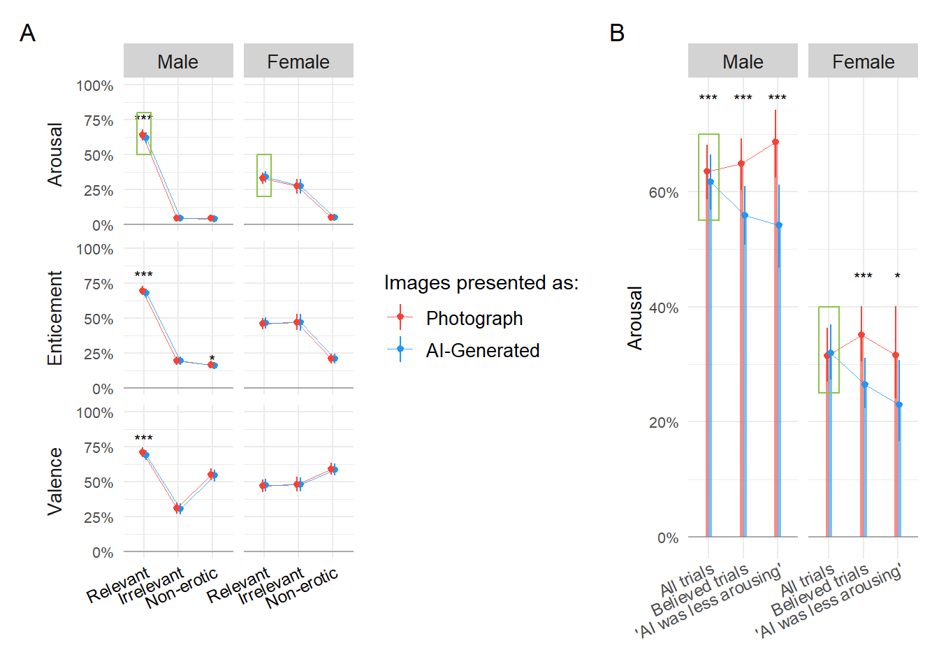

m6 <- glm(Feedback_AILessArousing ~ Sex / BAIT_Visual, 
    data=mutate(dfsub, Feedback_AILessArousing = ifelse(Feedback_AILessArousing=="True", 1, 0)), 
    family="binomial")

results_table(m6)

Parameter	Log-Odds	SE	95% CI	z	p
(Intercept)	-0.84	1.02	(-2.92, 1.12)	-0.82	0.412
Sex (Male)	0.44	1.20	(-1.89, 2.84)	0.36	0.716
Sex (Female) × BAIT Visual	-2.11	1.53	(-5.14, 0.88)	-1.39	0.166
Sex (Male) × BAIT Visual	-2.70	0.98	(-4.66, -0.79)	-2.74	0.006

pred3 <- estimate_relation(m6, length=50) 

p3 <- pred3 |> 
  mutate(Sex = fct_relevel(Sex, "Male", "Female")) |> 
  ggplot(aes(x=BAIT_Visual, y=Predicted)) +
  geom_hline(yintercept=0, color="darkgrey") +
  geom_ribbon(aes(ymin=CI_low, ymax=CI_high), alpha=0.3) + 
  geom_line() +
  geom_text(data=data.frame(Sex = as.factor("Male")), aes(x=0.65, y=0.25), label="**") +
  facet_grid(~Sex) +
  scale_y_continuous(labels=scales::percent, expand=c(0, 0)) +
  scale_x_continuous(breaks = c(0.3, 0.5, 0.7, 0.9)) +
  labs(y = "\nProbability of 'AI was less arousing' Feedback\n",
       x = "\nBeliefs about Artificial Information Technology (BAIT)\n'AI algorithms can generate realistic images'",
       tag = "C") +
  theme_minimal() +
  theme(strip.text = element_blank(),
        axis.text.y = element_text(size = 8),
        axis.title.y = element_text(size = 10),
        axis.text.x = element_text(size = 8),
        axis.title.x = element_text(size = 10))


p4 <- patchwork::wrap_plots(p2 / p3 + plot_layout(heights = c(1, 1.6)))
p <- patchwork::wrap_plots(p1 | p4, guides="collect")
p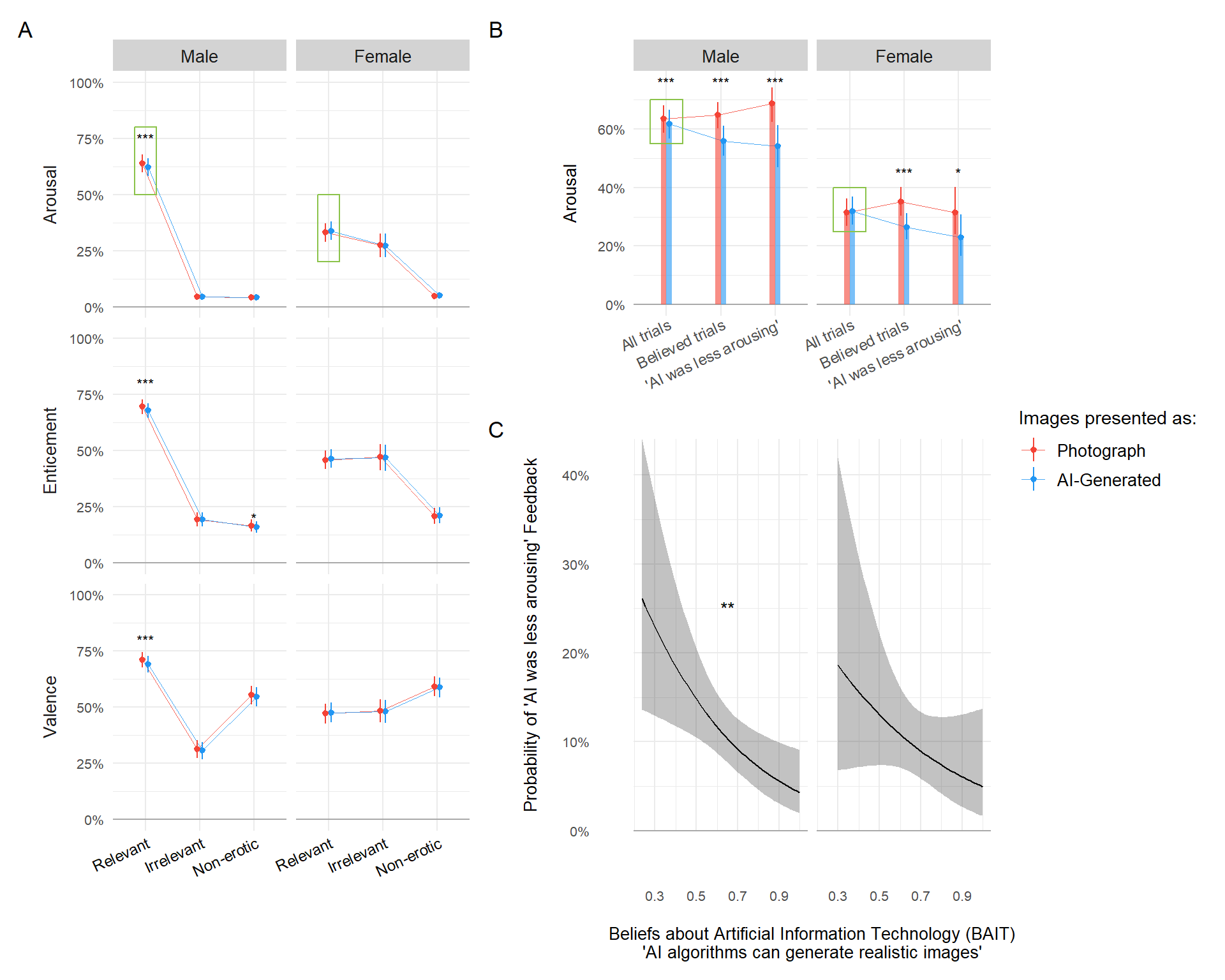

ggsave("figures/figure1.png", p, width=10, height=8, dpi=300)

m4 <- glmmTMB::glmmTMB(Arousal ~ SexualActivity / Sex / Condition + (Condition | Participant) + (1|Item),
                      data=filter(df, Relevance=="Relevant", ConditionBelief == "True"), 
                      family=glmmTMB::ordbeta(),
                      control = glmmTMB::glmmTMBControl(parallel = 8))

summary(m4)

pred3 <- estimate_relation(m4) 
pred3 |> 
  mutate(xnum = as.numeric(as.factor(SexualActivity))) |>
  ggplot(aes(x=SexualActivity, y=Predicted)) +
  # geom_ribbon(aes(x=xnum, ymin=CI_low, ymax=CI_high, fill=Condition), alpha=0.5) +
  geom_line(aes(group=Condition, color=Condition), position = position_dodge(width=0.2)) +
  geom_pointrange(aes(ymin = CI_low, ymax=CI_high, color=Condition), position = position_dodge(width=0.2)) +
  facet_grid(~Sex) 

m5 <- glmmTMB::glmmTMB(Arousal ~ Sex / (Condition * GAAIS_Negative) + (Condition | Participant) + (1|Item),
                      data=filter(df, Relevance=="Relevant", ConditionBelief == "True"), 
                      family=glmmTMB::ordbeta(),
                      control = glmmTMB::glmmTMBControl(parallel = 8))
summary(m5)

pred4 <- estimate_relation(m5, length=30) 
pred4 |> 
  ggplot(aes(x=GAAIS_Negative, y=Predicted)) +
  geom_line(aes(group=Condition, color=Condition)) +
  facet_grid(~Sex)