Analysis

Data Preparation

library(tidyverse)
library(easystats)
library(patchwork)
library(ggside)
library(dtwclust)

df <- rbind(
  read.csv("../data/data_hep1.csv"),
  read.csv("../data/data_hep2.csv"),
  read.csv("../data/data_hep3.csv"),
  read.csv("../data/data_hep4.csv"),
  read.csv("../data/data_hep5.csv"),
  read.csv("../data/data_hep6.csv"),
  read.csv("../data/data_hep7.csv"),
  read.csv("../data/data_hep8.csv"),
  read.csv("../data/data_hep9.csv"),
  read.csv("../data/data_hep10.csv"),
  read.csv("../data/data_hep11.csv"))

dfsub <- read.csv("https://raw.githubusercontent.com/RealityBending/InteroceptionPrimals/main/data/data_participants.csv") |> 
  rename(Participant="participant_id") |> 
  select(-matches("\\d"))

dffeat <- read.csv("../data/data_features.csv") |> 
  merge(select(dfsub, Participant, starts_with("MAIA_"), starts_with("IAS"), starts_with("HRV"), starts_with("HCT")), 
        by="Participant")

Exclusion

exclude <- c("sub-06", "sub-76", "sub-94")

dat <- df |>  
  summarize(ggdist::mean_qi(AF7, .width=0.2), .by=c("Participant", "Condition", "time")) |>
  mutate(Sensor = "AF7") |> 
  rbind(
    df |>  
      summarize(ggdist::mean_qi(AF8, .width=0.2), .by=c("Participant", "Condition", "time")) |>
      mutate(Sensor = "AF8")
  )

dat_rect <- summarize(dat, ymin = min(y), ymax = max(y), .by=c("Participant")) |> 
  mutate(Exclude = case_when(Participant %in% exclude ~ TRUE, .default = FALSE))

dat |>
  mutate(color = paste0(Condition, "_", Sensor)) |> 
  ggplot() +
  geom_vline(xintercept=0) +
  geom_vline(xintercept=c(-0.14, 0.1), color="grey") +
  geom_line(aes(x=time, y=y, color=color), linewidth=0.5) +
  geom_rect(data=dat_rect, aes(xmin=-0.3, xmax=0.8, ymin=ymin, ymax=ymax, color=Exclude), alpha=0, show.legend = FALSE) +
  scale_color_manual(values=c("RestingState_AF7"="dodgerblue", "RestingState_AF8"="darkblue", 
                              "HCT_AF7"="red", "HCT_AF8"="darkred", "TRUE"="red", "FALSE"="white"),
                     breaks=c("RestingState", "HCT")) +
  # geom_line(aes(color=Condition, group=epoch)) +
  facet_wrap(~Participant, scales="free_y", nrow=10) +
  theme_minimal() +
  theme(axis.text.y = element_blank(),
        axis.title.y = element_blank())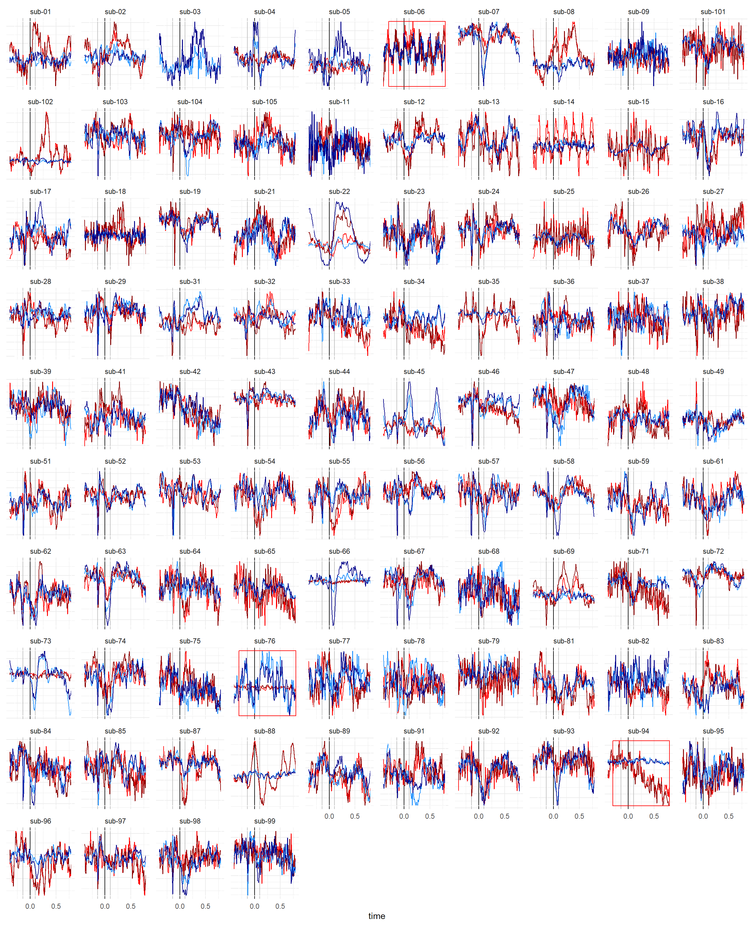

df <- filter(df, !Participant %in% exclude)
dffeat <- filter(dffeat, !Participant %in% exclude)
dfsub <- filter(dfsub, !Participant %in% exclude)

Sample

df |>  
  summarize(n = length(unique(epoch)), .by=c("Participant", "Condition")) |> 
  ggplot(aes(x=n, fill=Condition)) +
  geom_histogram(alpha=0.7, binwidth=30)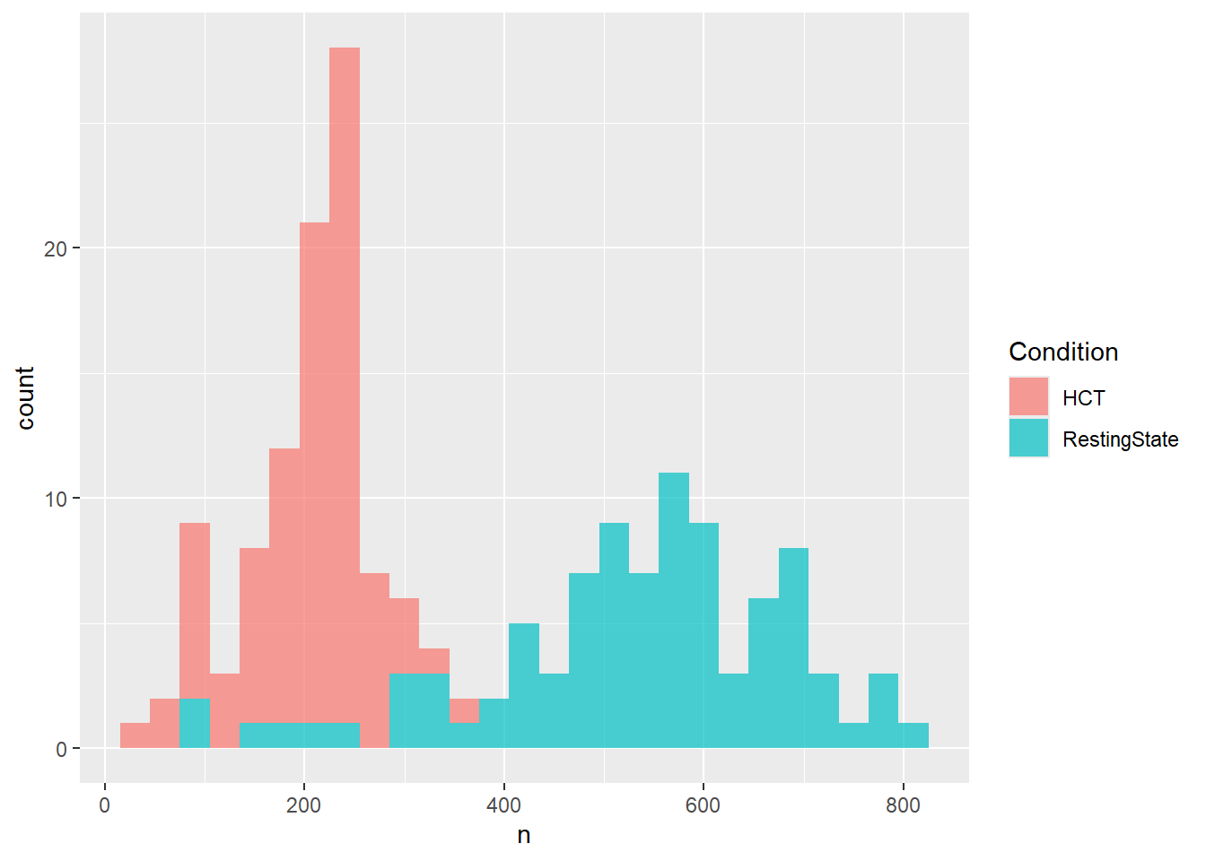

Grand Average

dfavsub <- df |>  
  summarize(AF7 = mean(AF7), AF8=mean(AF8), .by=c("Participant", "Condition", "time")) |> 
  summarize(AF7 = median(AF7), AF8=median(AF8), .by=c("Condition", "time")) |> 
  pivot_longer(c("AF7", "AF8"), names_to = "Sensor", values_to="EEG")

ecg <- summarize(df, ECG = median(ECG), RSP = median(RSP), .by="time") |> 
  mutate(ECG = datawizard::rescale(ECG, to=c(min(dfavsub$EEG), max(dfavsub$EEG))))

p1 <- dfavsub |> 
  mutate(Condition = str_replace(Condition, "RestingState", "Resting State"),
         Condition = str_replace(Condition, "HCT", "Heartbeat Counting")) |> 
  ggplot(aes(x=time, y=EEG)) +
  geom_vline(xintercept=0, color="grey") +
  geom_line(data=ecg, aes(y=ECG), color="red", linewidth=2, alpha=0.1) +
  geom_line(aes(color=Condition), linewidth=1) +
  scale_color_manual(values=c("Resting State"="#2196F3", "Heartbeat Counting"="#FF7811")) +
  scale_x_continuous(breaks = c(-0.4, -0.2, 0, 0.2, 0.4, 0.6, 0.8)) +
  facet_wrap(~Sensor) +
  theme_minimal() +
  theme(strip.background = element_rect(fill="grey", color=NA),
        axis.text.y = element_blank(),
        axis.title.x = element_blank(),
        axis.title.y = element_blank(),
        panel.grid.minor = element_blank(),
        plot.title = element_text(face="bold", hjust=0.5)) +
  labs(title="Heartbeat Evoked Potentials", x="Time")
p1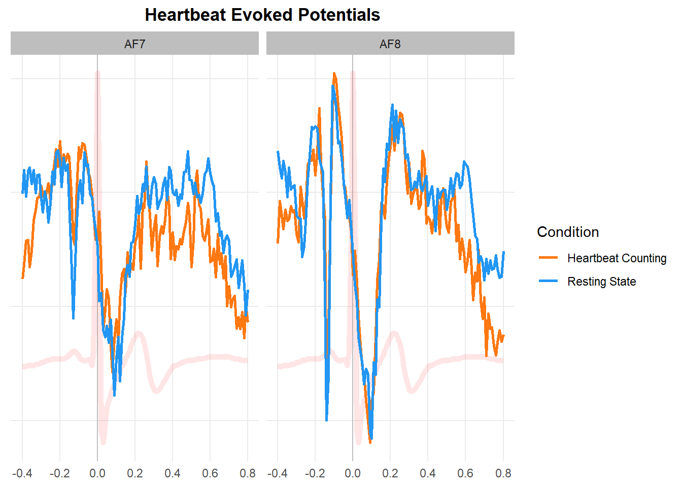

Rolling correlations

HCT

dfrollr <- data.frame()
for(w in unique(dffeat$time)) {
  for(c in unique(dffeat$Condition)) {
    dat <- dffeat[dffeat$time == w & dffeat$Condition == c, ]
    r <- correlation(select(dat, starts_with("AF")),
                     select(dat, starts_with("MAIA"), starts_with("IAS"), starts_with("HRV"), starts_with("HCT")),
                     p_adjust="none") |> 
      separate(Parameter1, into=c("Sensor", "Type", "Feature")) |> 
      mutate(time = w,  Condition = c)
    dfrollr <- rbind(dfrollr, r)
  }
}

make_rollingplot <- function(dfrollr, legend.position="top") {
  dfrollr |>
    mutate(Condition = str_replace(Condition, "RestingState", "RS"),
           color = paste0(Feature, " (", Condition, ")"),
           color = fct_rev(color),
           alpha = ifelse(p < .05, "Sig", "Nonsig"))  |> 
    ggplot(aes(x=time, y=r)) +
    geom_hline(yintercept = 0) +
    geom_vline(xintercept = 0, color="grey") +
    geom_line(aes(color=color, alpha=alpha, group=color), linewidth=1) +
    scale_alpha_manual(values=c("Sig"=1, "Nonsig"=0.3), guide="none") +
    # scale_color_manual(values = c("ERP_Mean_RestingState" = "#F44336", "ERP_Mean_HCT" = "#C62828",
    #                               "ERP_Median_RestingState" = "#2196F3", "ERP_Median_HCT" = "#1565C0")) +
    scale_x_continuous(breaks = c(-0.4, -0.2, 0, 0.2, 0.4, 0.6, 0.8)) +
    facet_grid(Parameter2~Sensor, switch="y") +
    theme_minimal() +
    theme(strip.background.x = element_blank(),
          strip.text.x = element_blank(),
          # strip.background.x = element_rect(fill="grey", color=NA),
          strip.placement = "outside", 
          axis.title.y = element_blank(),
          panel.grid.minor = element_blank(),
          plot.title = element_text(face="bold", hjust=0.5),
          legend.position = legend.position) +
    coord_cartesian(xlim = c(-0.4, 0.8)) +
    labs(color="Feature", x="Time")
}

make_rollingplot(filter(dfrollr, Feature == "Mean", str_detect(Parameter2, "HCT_"))) |
  make_rollingplot(filter(dfrollr, Feature == "Median", str_detect(Parameter2, "HCT_")))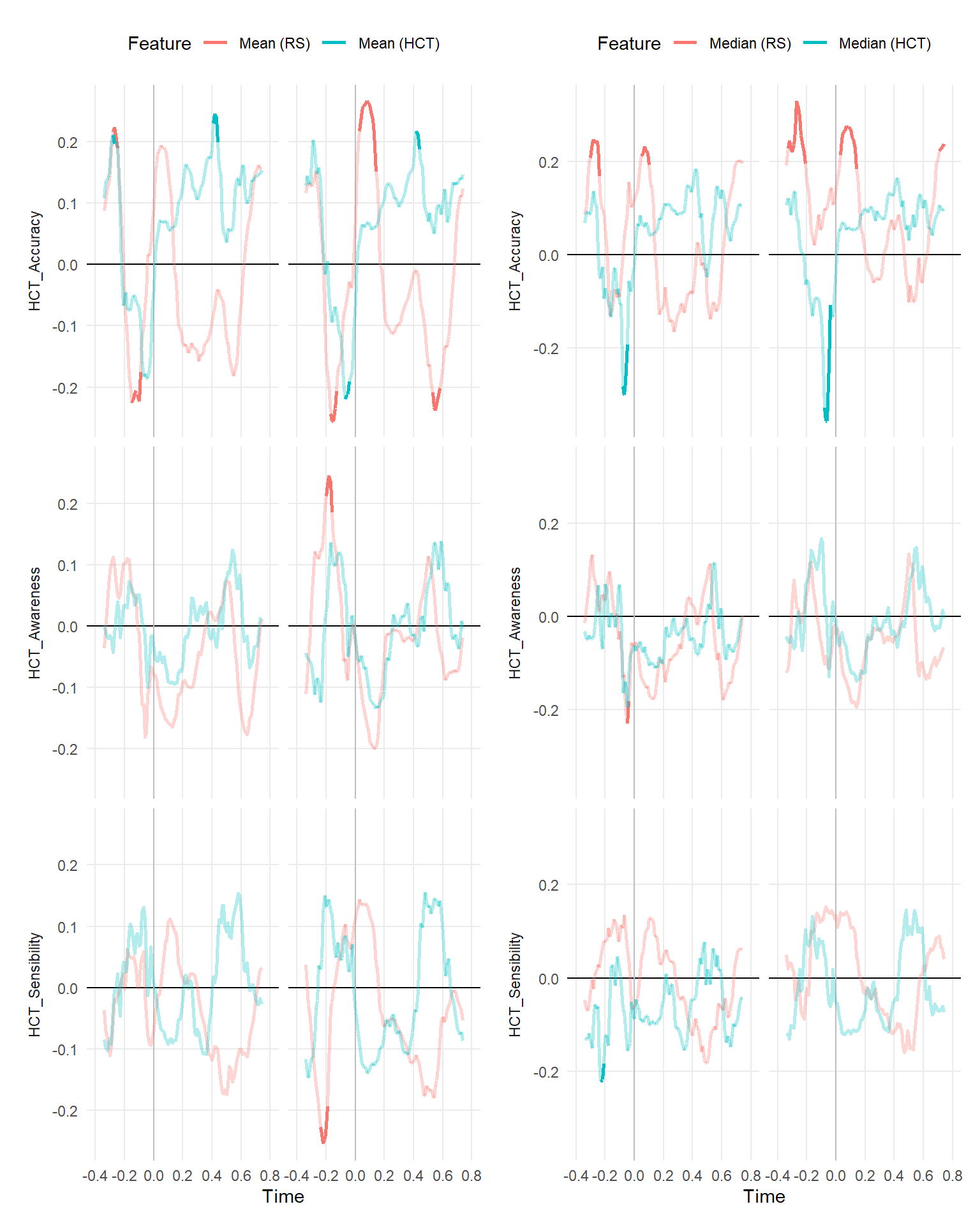 

make_rollingplot(filter(dfrollr, str_detect(Feature, "1015Mean|1530Mean|1030Mean"), str_detect(Parameter2, "HCT_")))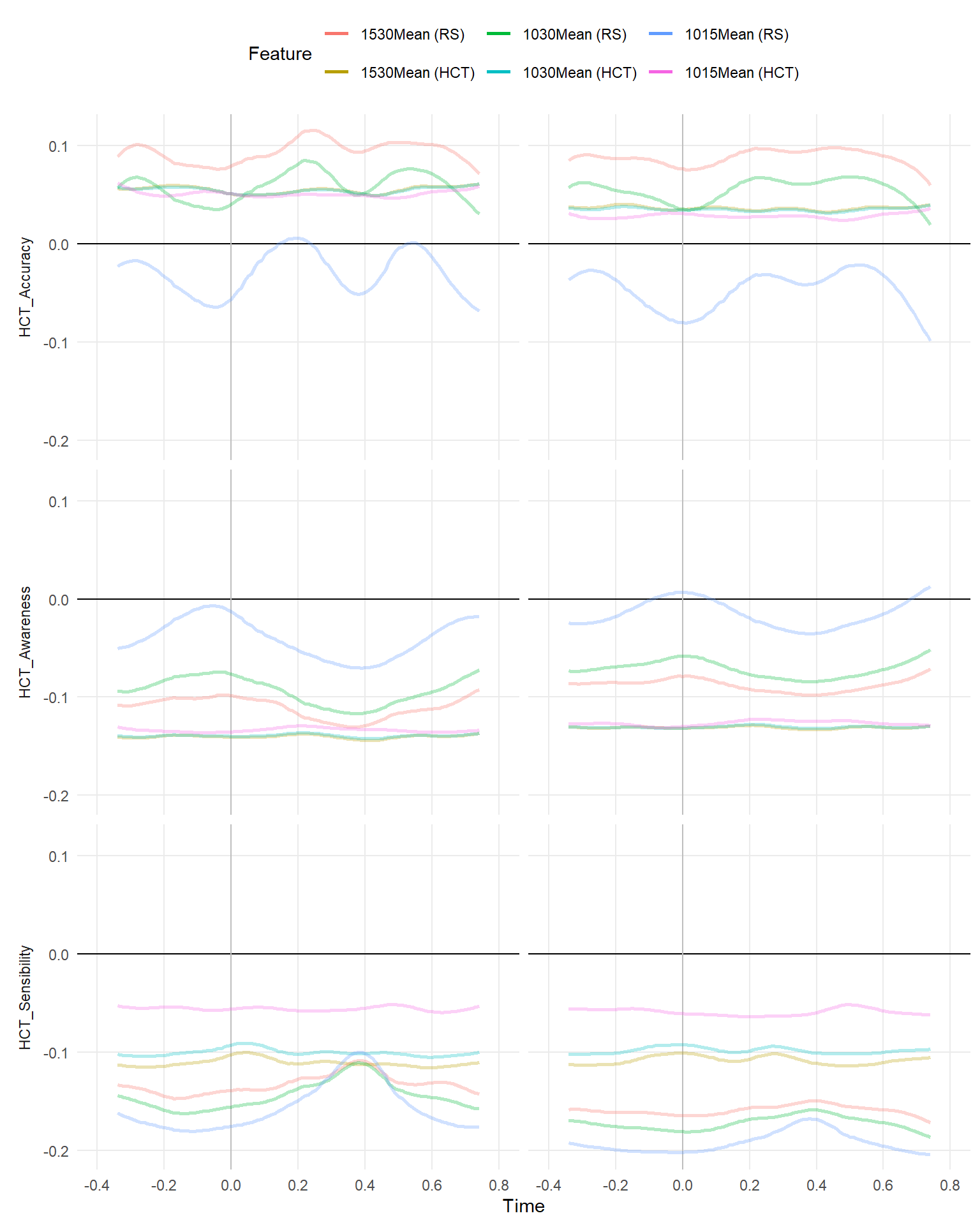 

make_rollingplot(filter(dfrollr, Type == "Fractal", str_detect(Parameter2, "HCT_"))) |
  make_rollingplot(filter(dfrollr, Type == "Entropy", str_detect(Parameter2, "HCT_")))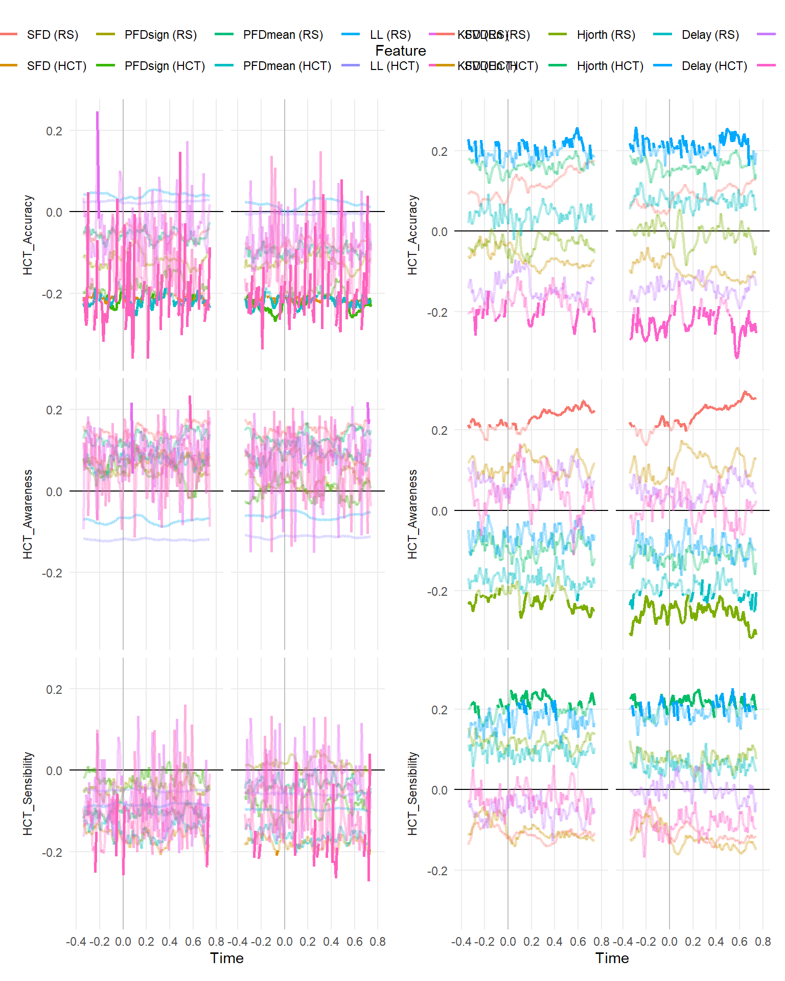

Scales

make_rollingplot(filter(dfrollr, Feature == "Mean", str_detect(Parameter2, "MAIA|IAS"))) |
  make_rollingplot(filter(dfrollr, Feature == "Median", str_detect(Parameter2, "MAIA|IAS")))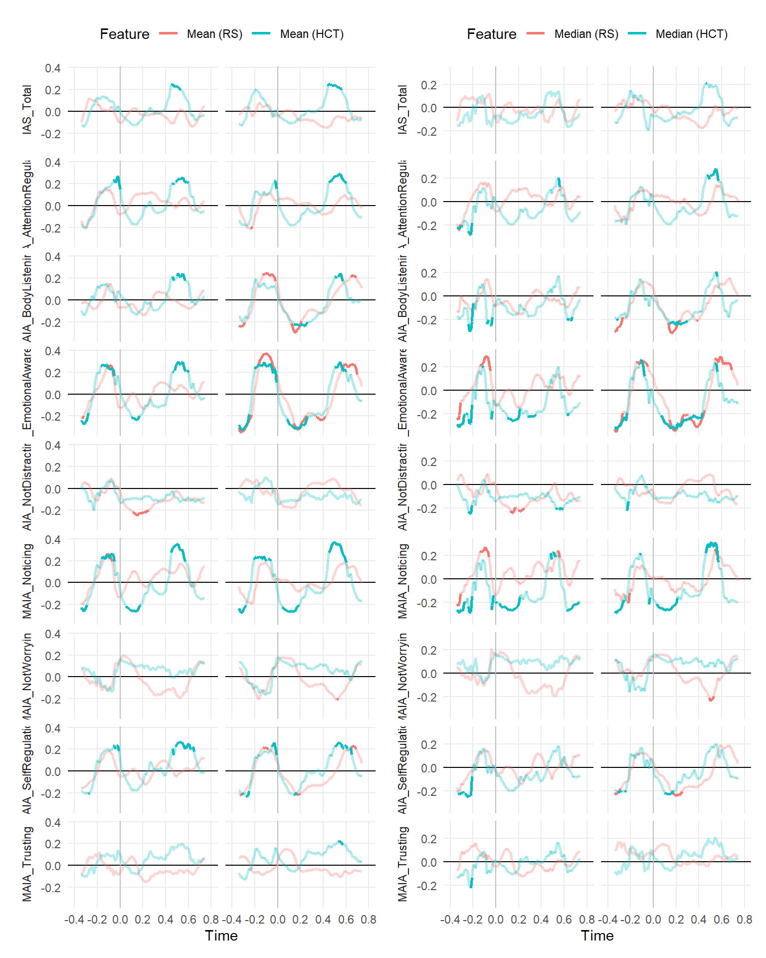

make_rollingplot(filter(dfrollr, str_detect(Feature, "1015Mean|1530Mean|1030Mean"), str_detect(Parameter2, "MAIA|IAS"))) 

make_rollingplot(filter(dfrollr, Type == "Fractal", str_detect(Parameter2, "MAIA|IAS"))) |
  make_rollingplot(filter(dfrollr, Type == "Entropy", str_detect(Parameter2, "MAIA|IAS")))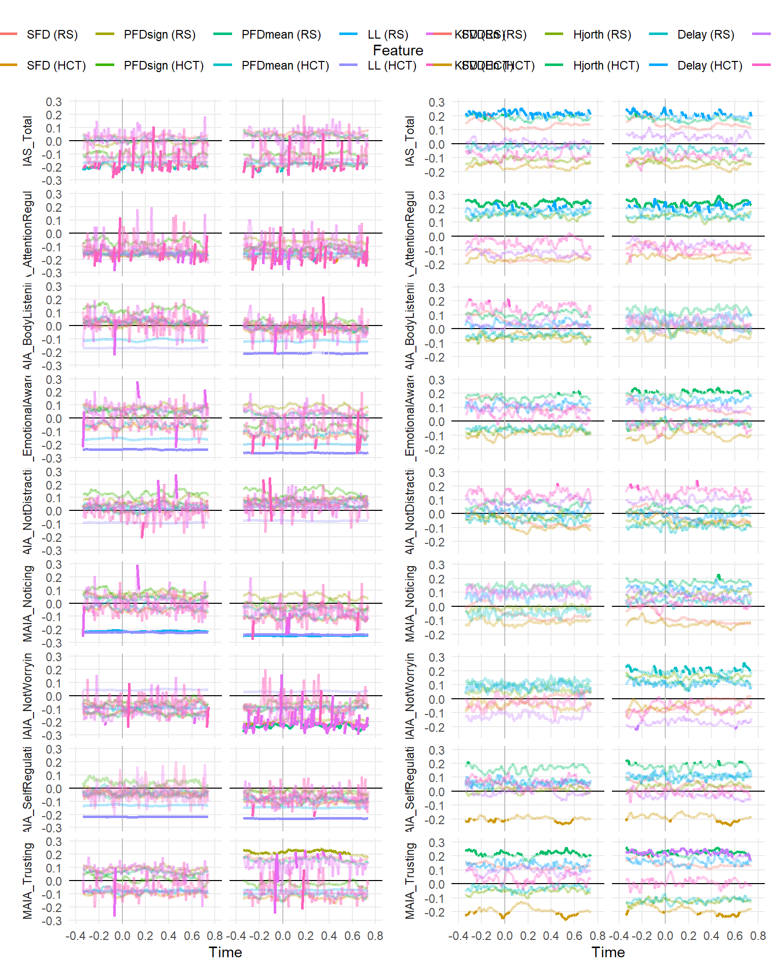

HRV

make_rollingplot(filter(dfrollr, Feature == "Mean", str_detect(Parameter2, "HRV"))) | 
  make_rollingplot(filter(dfrollr, Feature == "Median", str_detect(Parameter2, "HRV")))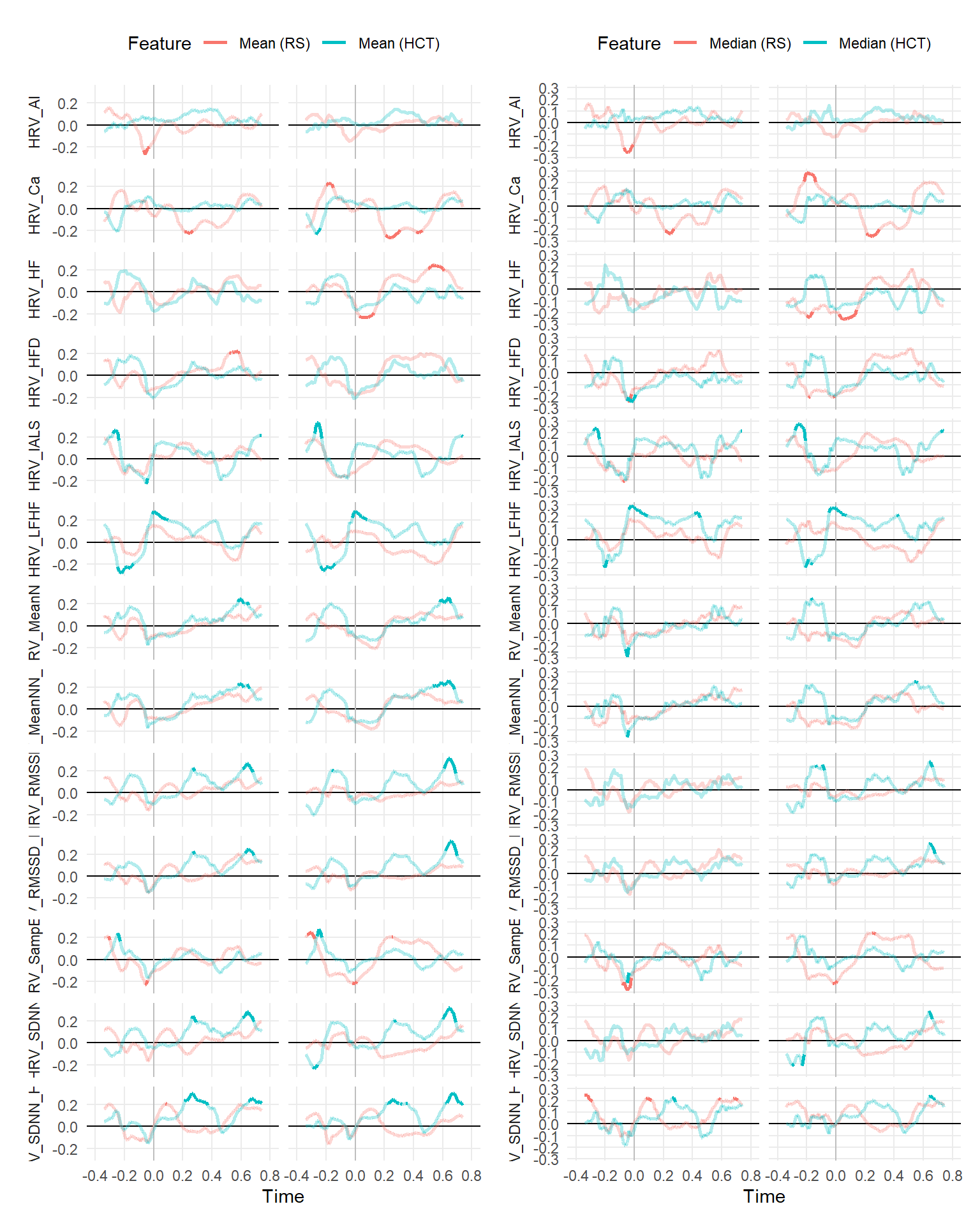

make_rollingplot(filter(dfrollr, str_detect(Feature, "1015Mean|1530Mean|1030Mean"), str_detect(Parameter2, "HRV")))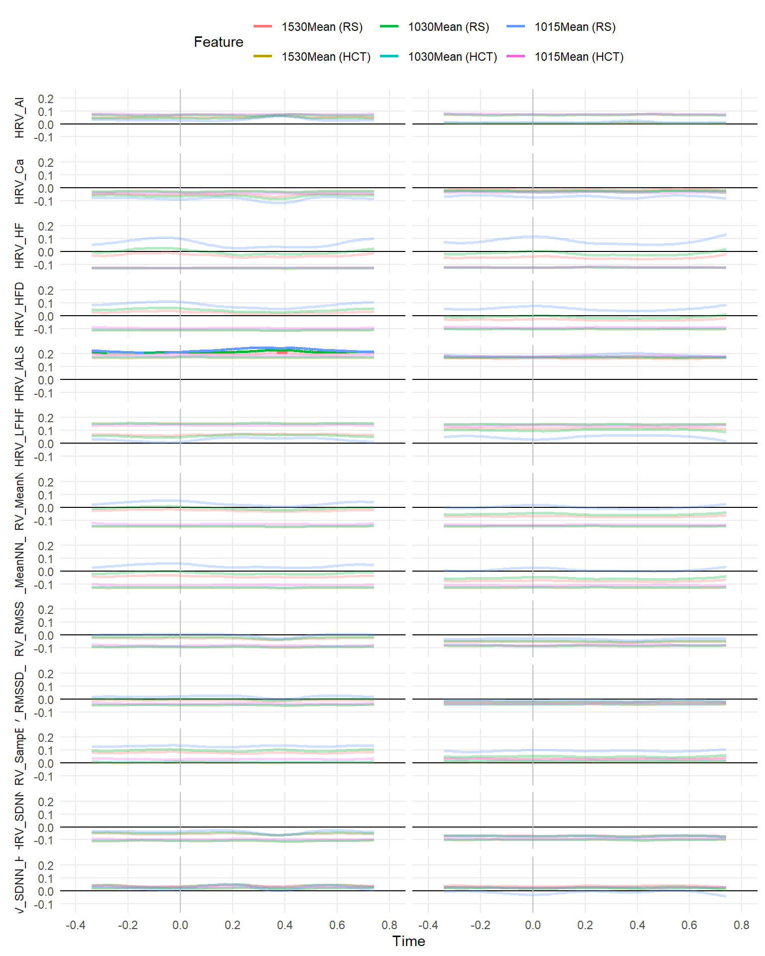 

make_rollingplot(filter(dfrollr, Type == "Fractal", str_detect(Parameter2, "HRV"))) |
  make_rollingplot(filter(dfrollr, Type == "Entropy", str_detect(Parameter2, "HRV")))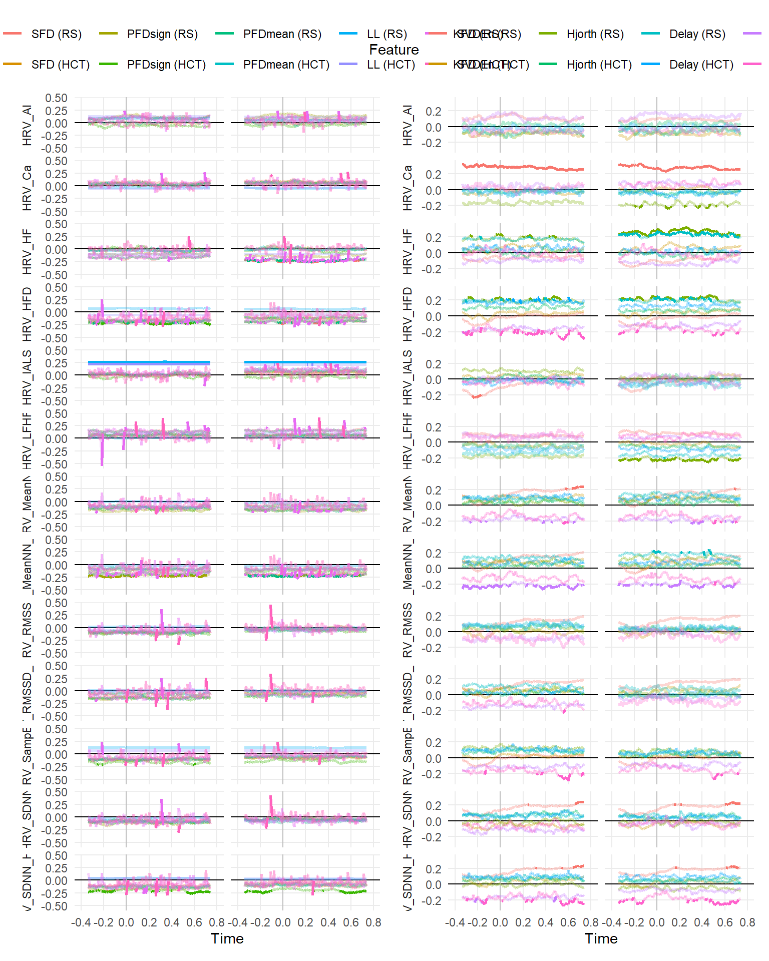

dfrollr |> 
  mutate(Feature = fct_reorder(Feature, abs(r)), 
         sig=ifelse(p < .05, "Sig", "Nonsig")) |> 
  ggplot(aes(x=abs(r), y=Feature, fill=sig)) +
  ggdist::stat_slabinterval()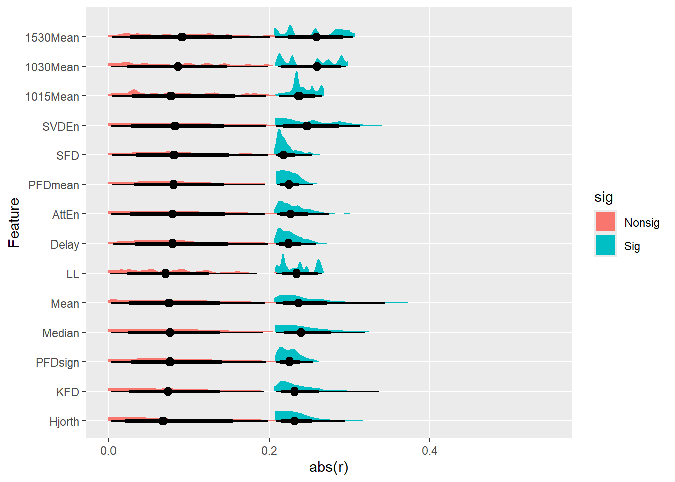

df_p <- dfrollr |>
  filter(str_detect(Parameter2, "HCT_|EmotionalAwareness|Noticing|IALS|RMSSD$")) |>
  mutate(Feature = str_replace(Feature, "1530Mean", "Power 15-30Hz"),
         Parameter2 = str_replace(Parameter2, "HCT_Accuracy", "HCT - Acc"),
         Parameter2 = str_replace(Parameter2, "HCT_Awareness", "HCT - Awa"),
         Parameter2 = str_replace(Parameter2, "HCT_Sensibility", "HCT - Sen"),
         Parameter2 = str_replace(Parameter2, "HRV_MeanNN", "HRV - MeanNN"),
         Parameter2 = str_replace(Parameter2, "HRV_RMSSD", "HRV - RMSSD"),
         Parameter2 = str_replace(Parameter2, "HRV_IALS", "HRV - IALS"),
         Parameter2 = str_replace(Parameter2, "MAIA_EmotionalAwareness", "MAIA - EmoAwa"),
         Parameter2 = str_replace(Parameter2, "MAIA_Noticing", "MAIA - Noticing"))


p2 <- filter(df_p, Feature %in% c("Mean")) |>
  make_rollingplot(legend.position="right") +
  scale_color_manual(values = c("Mean (RS)" = "#2196F3", "Mean (HCT)" = "#FF7811"))

p1 / p2 + plot_layout(heights=c(0.35, 0.75))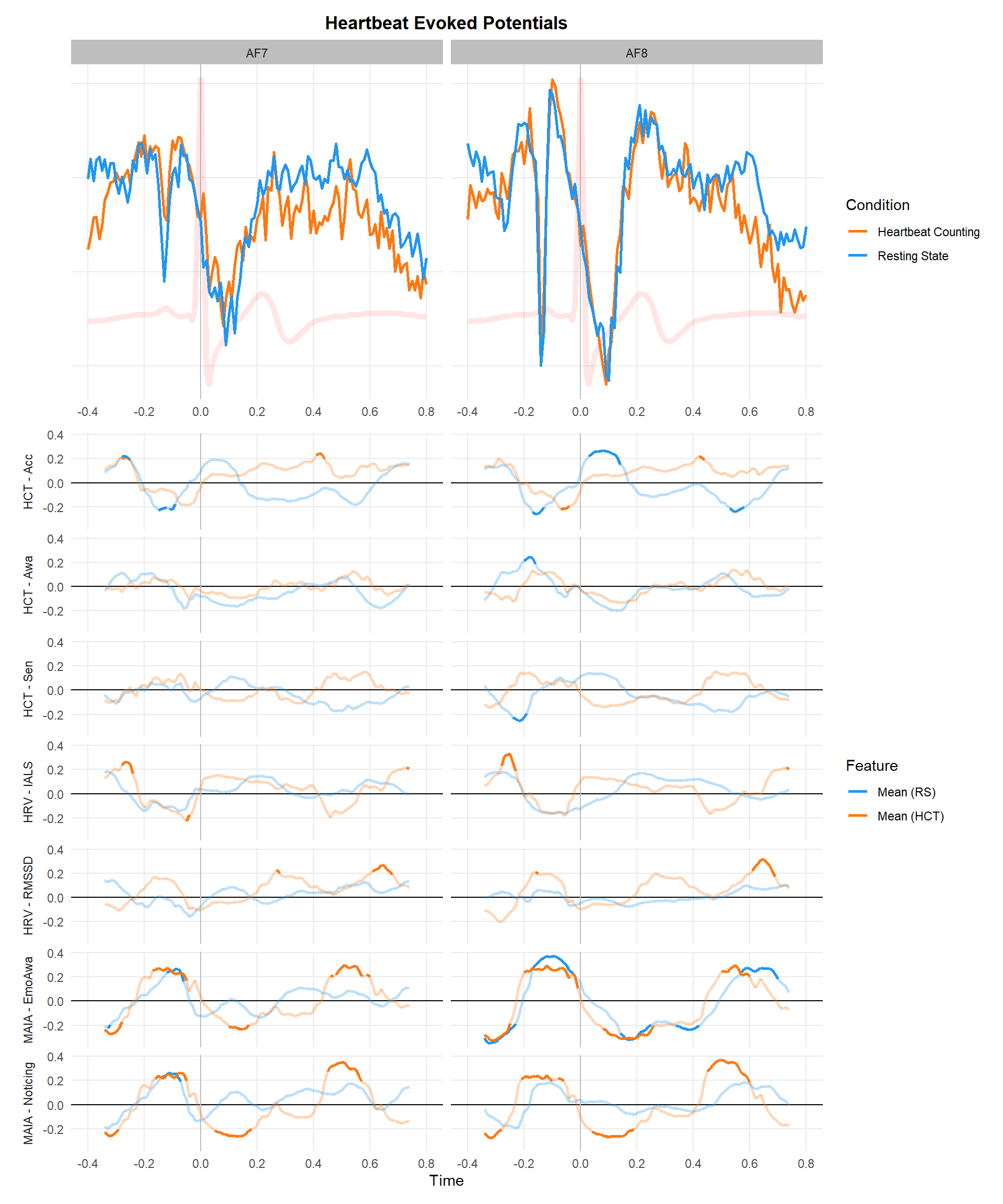

p3 <- filter(df_p, Feature %in% c("PFDmean", "Power 15-30Hz", "SVDEn", "Hjorth", "LL")) |>
  make_rollingplot(legend.position="right") +
  scale_color_manual(values = c("SVDEn (RS)" = "#4CAF50", "SVDEn (HCT)" = "#1B5E20",
                                "Hjorth (RS)" = "#FF9800", "Hjorth (HCT)" = "#E65100",
                                "Power 15-30Hz (RS)" = "#2196F3", "Power 15-30Hz (HCT)" = "#1565C0",
                                "PFDmean (RS)" = "#9C27B0", "PFDmean (HCT)" = "#4A148C",
                                "LL (RS)" = "#795548", "LL (HCT)" = "#4E342E")) +
  ggtitle("Frequency and Complexity Indices")
p3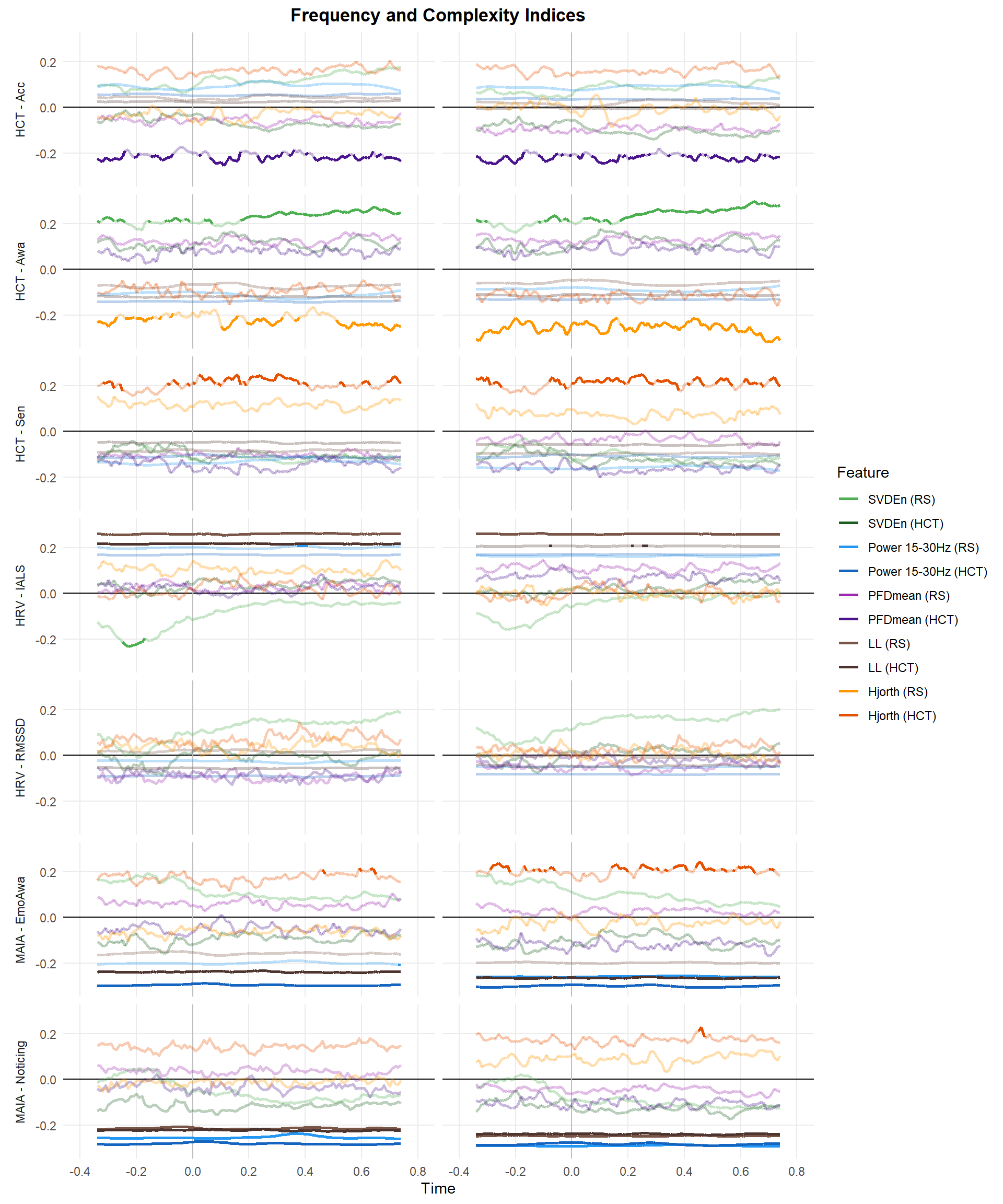

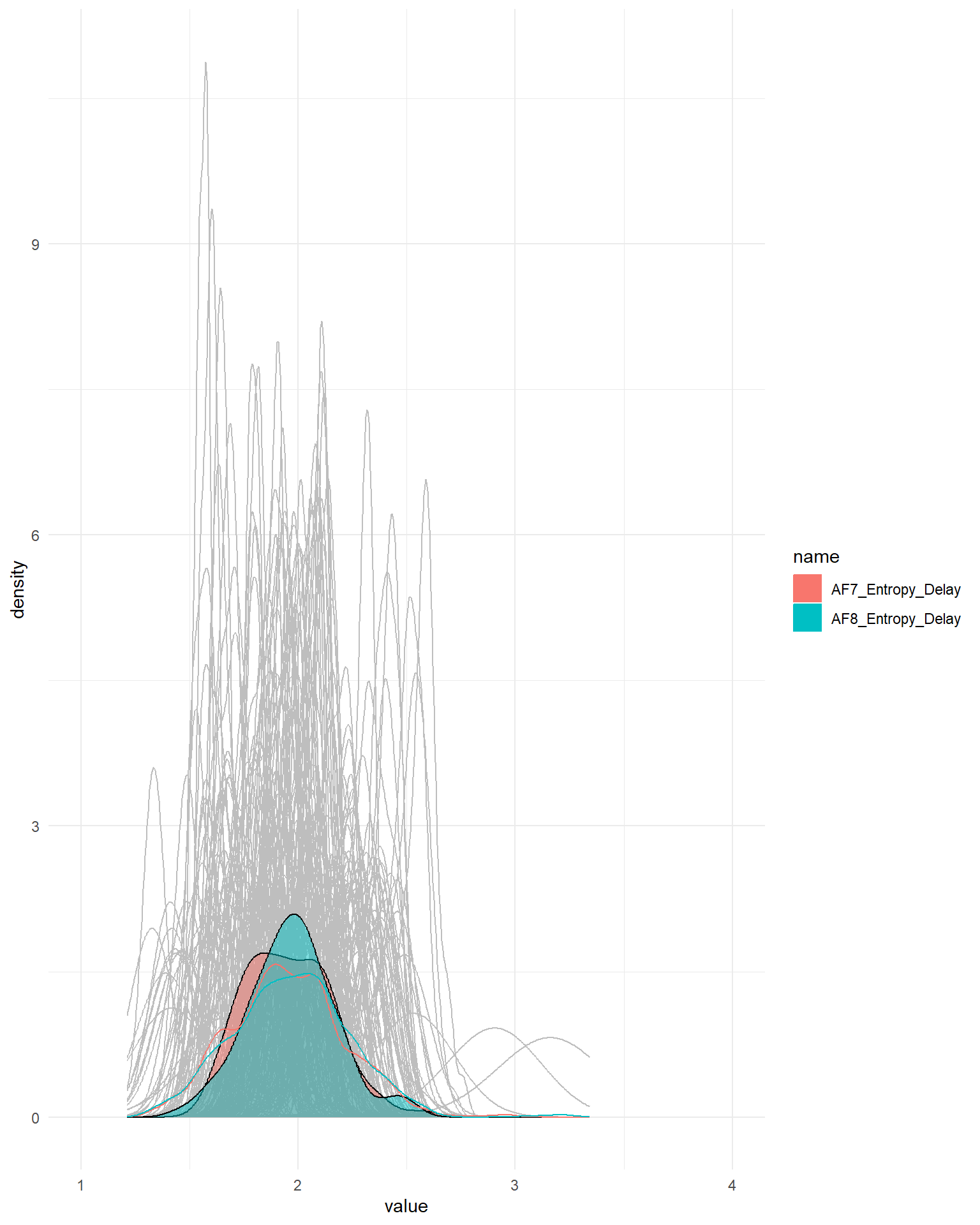
Index Validation

Complexity Parameters

delay <- dffeat |> 
  select(Participant, ends_with("Delay")) |> 
  pivot_longer(-Participant) 

 
summarize(delay, value = mean(value), .by=c("Participant", "name")) |> 
  ggplot(aes(x=value)) +
  geom_density(data=delay, aes(group=interaction(name, Participant)), alpha=0.5, color="grey") +
  geom_density(aes(fill=name), alpha=0.5) +
  geom_density(data=delay, aes(color=name)) +
  coord_cartesian(xlim=c(1, 4)) +
  theme_minimal()

• What window maximizes correlations?
• Reliability as a function of number of epochs