Interoception Scale - Data Cleaning

Data Preparation

library(tidyverse)
library(easystats)
library(patchwork)
library(ggside)
library(ggdist)

df <- read.csv("../data/rawdata_participants.csv")

Feedback

Experiment Enjoyment

Code

df |> 
  summarise(n = n(), .by=c("Condition", "Experiment_Enjoyment")) |>
  filter(!is.na(Experiment_Enjoyment)) |> 
  mutate(n = n / sum(n),
         Experiment_Enjoyment = fct_rev(as.factor(Experiment_Enjoyment)),
         .by="Condition") |>
  ggplot(aes(y = Condition, x = n, fill = Experiment_Enjoyment)) +
  geom_bar(stat="identity", position="stack") +
  scale_fill_manual(values=c("green", "yellowgreen",  "yellow", "orange", "red")) +
  scale_x_continuous(expand=c(0, 0))  +
  labs(title="Experiment Enjoyment",
       subtitle="Proportion of participants by condition") + 
  guides(fill = guide_legend(reverse=TRUE)) +
  theme_minimal() +
  theme(axis.title.x = element_blank(),
        axis.text.x = element_blank(),
        legend.position = "top",
        legend.title = element_blank())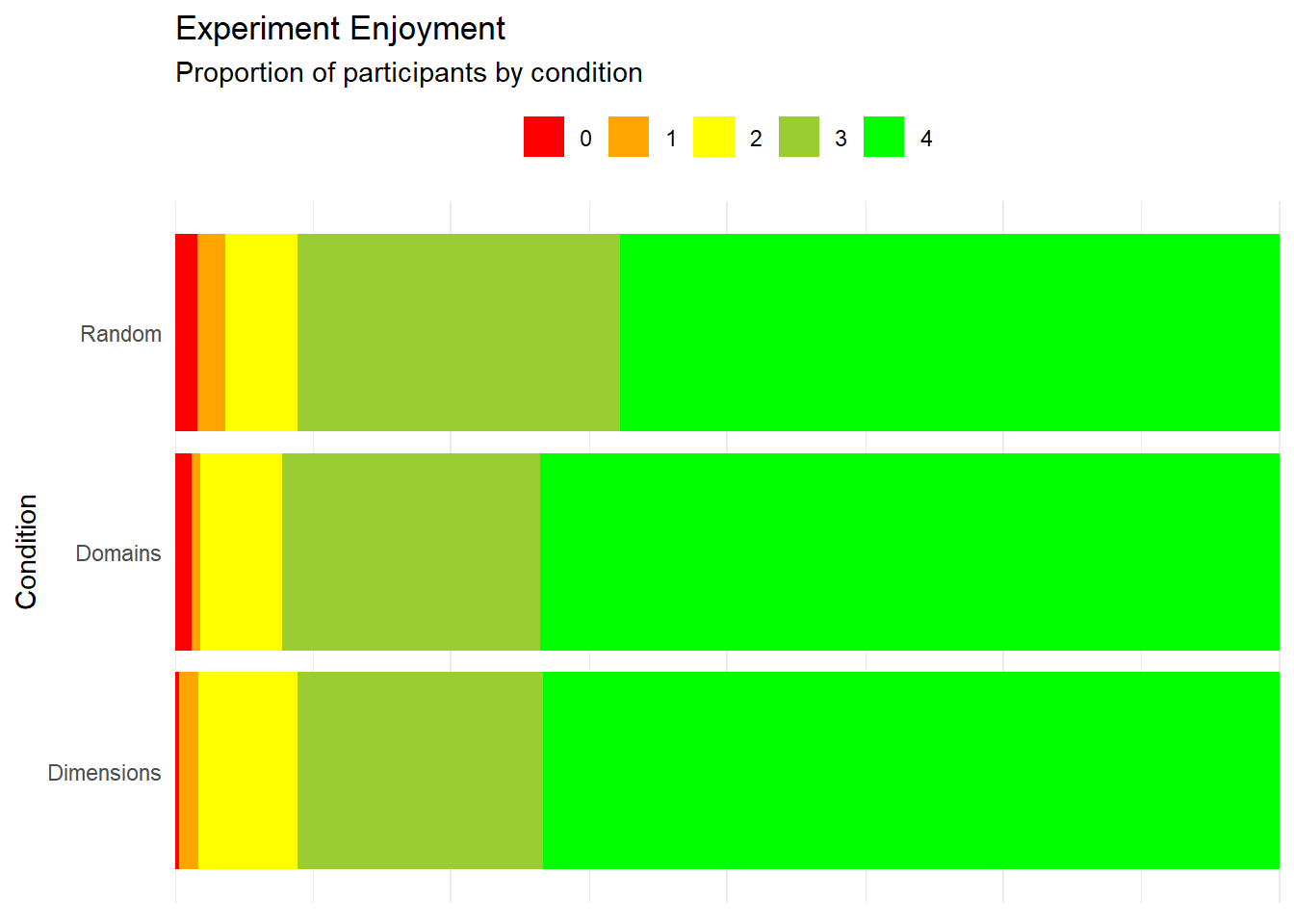

Code

lm(Experiment_Enjoyment ~ Condition, data = df) |> 
  modelbased::estimate_contrasts(p_adjust="none", contrast = "Condition") |> 
  display()

Marginal Contrasts Analysis
Level1	Level2	Difference	SE	95% CI	t(731)	p
Domains	Dimensions	3.16e-03	0.07	(-0.14, 0.15)	0.04	0.966
Random	Dimensions	-0.11	0.07	(-0.26, 0.04)	-1.48	0.140
Random	Domains	-0.11	0.07	(-0.26, 0.03)	-1.55	0.121

Variable predicted: Experiment_Enjoyment; Predictors contrasted: Condition; p-values are uncorrected.

Comments

Code

data.frame(Comments = df$Experiment_Feedback) |> 
  filter(!tolower(Comments) %in% c(NA, "no", "none", "no thank you", "no not at all", "no thanks", "no comment", "nil", "n.a", "n/a", "na", "not really", "thank you", "nothing", "no not at the moment", "none for now", "thank you!", "thanks", "not really.")) |> 
  gt::gt() |> 
  gt::opt_stylize() |> 
  gt::opt_interactive(use_compact_mode = TRUE)

Exclusions

Code

outliers <- list()

Attention Checks

Code

dfchecks <- df |>
  dplyr::mutate(
    # "I always know that I am attentively doing a study"
    A1 = ifelse(Sexual_State_A == 6 | Sexual_State_A == 5, 0, 1),
    # "Even if I am anxious, I should now answer all the way to the left"
    A2 = ifelse(Anxious_SkinThermo_A == 0, 0, 1),
    # "I often experience sensations, and I will answer zero to this question"
    A3 = ifelse(Nociception_ColonBladder_A == 0, 0, 1),
    # "In general, I am very sensitive and attentive to the questions I am currently answering"
    A4 = ifelse(Sensitivity_Cardiac_A == 6 | Sensitivity_Cardiac_A == 5, 0, 1),
    # "I often pay attention to the answers I am giving"
    A5 = ifelse(Sensitivity_Gastric_A == 6 | Sensitivity_Gastric_A == 5, 0, 1),
    # "I can always accurately answer to the left on this question to show that I am reading it"
    A6 = ifelse(Accuracy_Respiratory_A == 0 | Accuracy_Respiratory_A == 1, 0, 1),
    # "I can always accurately perceive that to this question I should answer the lowest option"
    A7 = ifelse(Accuracy_Genital_A == 0, 0, 1),
    # "Sometimes I notice that I need to answer all the way to the right"
    A8 = ifelse(Confusion_ColonBladder_A == 6, 0, 1),
    .keep = "none"
  ) 
dfchecks$Total <- rowSums(dfchecks)


dfchecks |>
  mutate(Total = as.factor(paste0(Total, "/8"))) |> 
  ggplot(aes(x = Total)) +
  geom_bar(aes(fill = Total)) +
  scale_fill_viridis_d(guide = "none") +
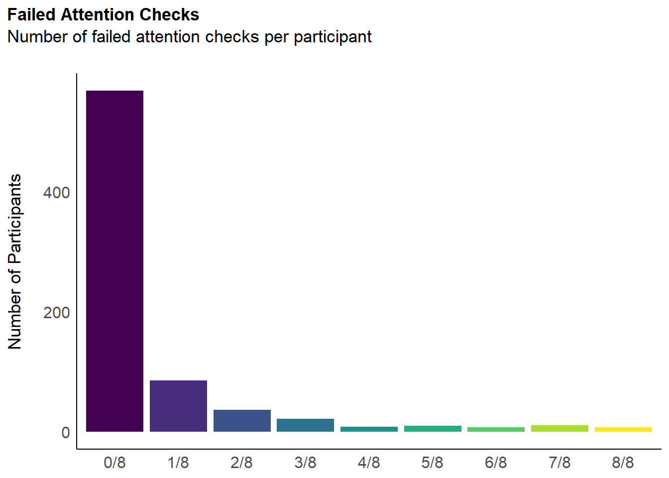
  labs(title = "Failed Attention Checks", y = "Number of Participants", subtitle = "Number of failed attention checks per participant") +
  theme_modern(axis.title.space = 15) +
  theme(
    plot.title = element_text(size = rel(1.2), face = "bold", hjust = 0),
    plot.subtitle = element_text(size = rel(1.2), vjust = 7),
    axis.title.x = element_blank(),
  )

Code

outliers$attentionchecks <- df$Participant[dfchecks$Total >= 1]

We removed 191 (25.13%) participants for having failed at least 1 attention check (out of 8).

Experiment Duration

Code

dfchecks$Duration <- df$Experiment_Duration
dfchecks$Outlier <- ifelse(dfchecks$Total >= 1, 1, 0)
dfchecks <- filter(dfchecks, Duration < 45)

m <- mgcv::gam(Outlier ~ s(Duration), data = dfchecks, family = "binomial")

estimate_relation(m, length=50) |> 
  ggplot(aes(x = Duration, y = Predicted)) +
  geom_ribbon(aes(ymin = CI_low, ymax = CI_high), alpha = 0.2) +
  geom_line() +
  geom_vline(xintercept=5, linetype="dashed", color="red") +
  theme_minimal() +
  ggside::geom_xsidedensity(data=mutate(dfchecks, 
                                        Outlier=ifelse(Outlier==1, "Failed attention check", "Valid")), 
                            aes(fill=Outlier), alpha=0.3) +
  ggside::theme_ggside_void() +
  labs(title = "Experiment Duration",
       subtitle = "Predicted probability of failing attention checks by duration",
       x = "Experiment Duration (minutes)",
       y = "Probability of failing attention checks")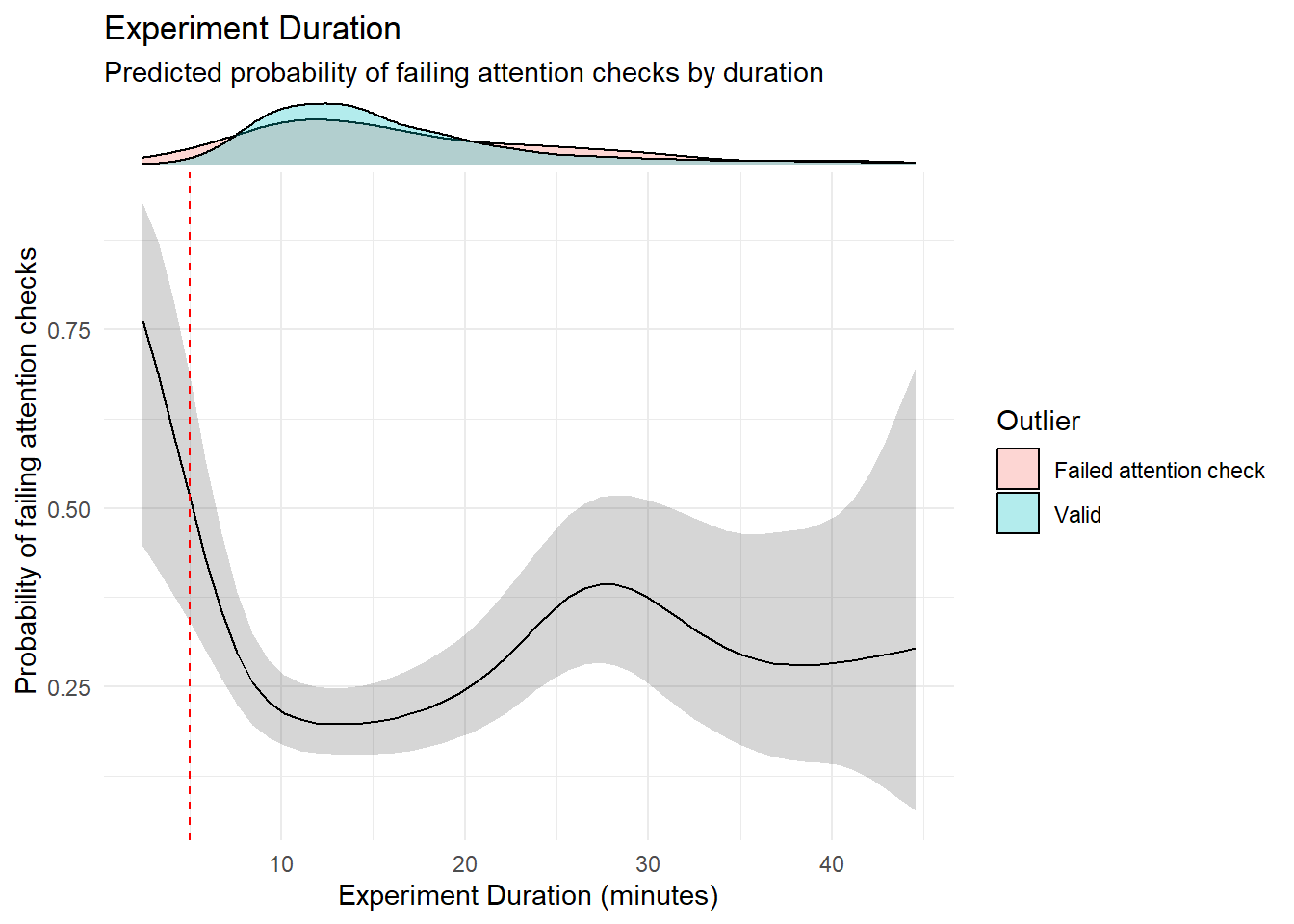

Code

outliers$duration <- as.character(df[df$Experiment_Duration < 5, "Participant"])
outliers$duration <- outliers$duration[!outliers$duration %in% outliers$attentionchecks]

We removed 0 (0.00%) participants for having completed the experiment in less than 5 minutes.

Multivariate Distance

Code

# Compute distance
dfoutlier <- performance::check_outliers(select(df, contains("_Q")), 
                                         method=c("optics"),
                                         threshold=list(optics=2.5, optics_xi=0.03)) |> 
  as.data.frame() |> 
  mutate(Participant = fct_reorder(df$Participant, Distance_OPTICS),
         Outlier_AttentionCheck = ifelse(Participant %in% outliers$attentionchecks, 1, 0),
         Outlier_Duration = ifelse(Participant %in% outliers$duration, 1, 0),
         Outlier = ifelse(Outlier_AttentionCheck == 1, "Failed Attention Checks", "Passed"),
         Outlier = ifelse(Outlier == "Passed" & Outlier_Duration == 1, "Duration", Outlier))


outliers$distance <- as.character(dfoutlier[dfoutlier$Distance_OPTICS < 12.5, "Participant"])
outliers$distance <- outliers$distance[!outliers$distance %in% c(outliers$attentionchecks, outliers$duration)]


p1 <- dfoutlier |> 
  ggplot(aes(x=Participant, y=Distance_OPTICS)) +
  geom_bar(aes(fill=Outlier), stat="identity") +
  geom_hline(yintercept = 12.5, linetype="dashed", color="red") +
  labs(fill = "Status") +
  theme_minimal() +
  theme(axis.text.x = element_blank(),
        panel.grid.major.x = element_blank())

m <- mgcv::gam(Outlier_AttentionCheck ~ s(Distance_OPTICS), data = dfoutlier, family = "binomial")
# parameters::parameters(m)

p2 <- estimate_relation(m, length=30) |> 
  ggplot(aes(x=Distance_OPTICS, y=Predicted)) +
  geom_ribbon(aes(ymin=CI_low, ymax=CI_high), alpha=0.2) +
  geom_line() +
  geom_vline(xintercept=12.5, linetype="dashed", color="red") +
  theme_minimal() 

p1 | p2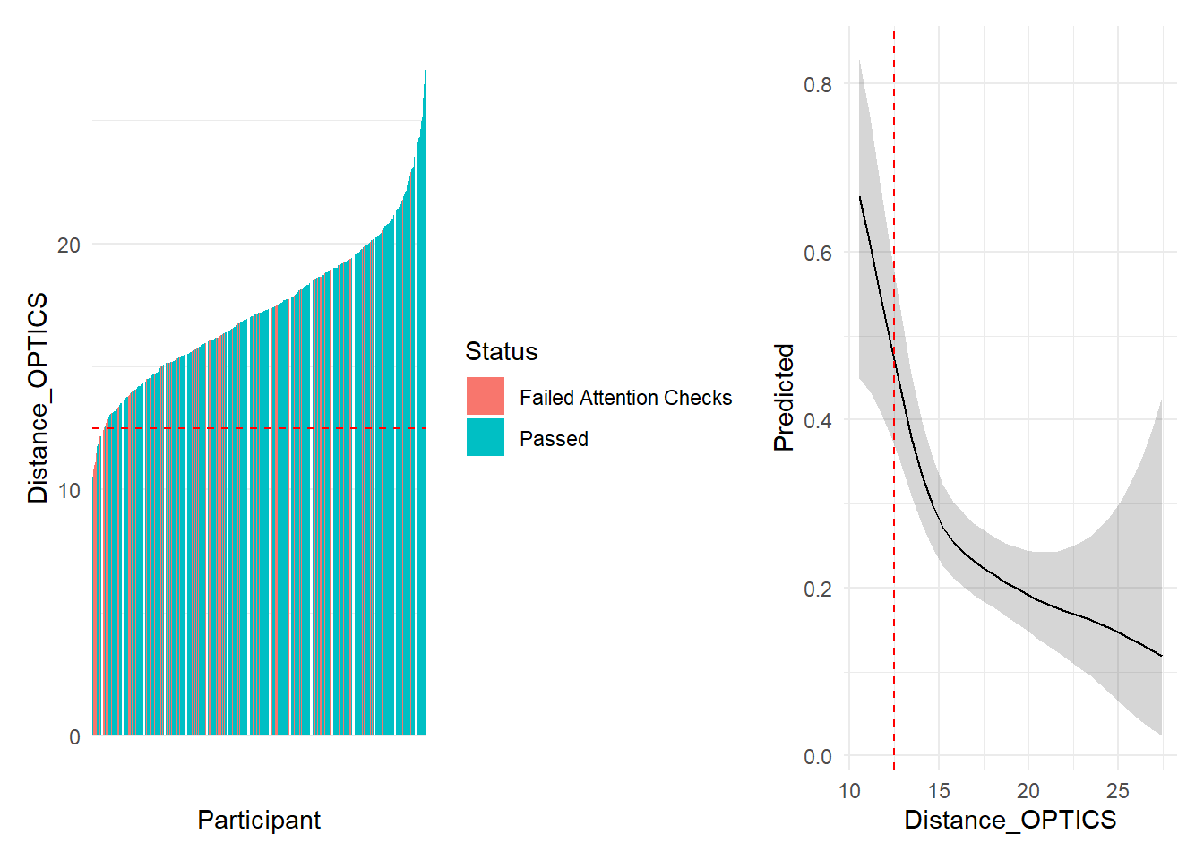

TODO: describe OPTICS.

We removed 10 (1.32%) participants based on multivariate distance.

Code

r_full <- cor(select(df, contains("_Q")))
r_cleaned <- filter(df, !Participant %in% c(outliers$attentionchecks, outliers$duration, outliers$distance)) |> 
  select(contains("_Q")) |> 
  cor()

data.frame(Full=r_full[lower.tri(r_full)], Clean=r_cleaned[lower.tri(r_cleaned)]) |> 
  pivot_longer(everything()) |> 
  ggplot(aes(x=value)) +
  geom_histogram(aes(fill=name, color=name), bins=60, alpha=0.3, position="identity") +
  theme_minimal()

df <- filter(df, !Participant %in% c(outliers$attentionchecks, outliers$duration, outliers$distance))

Final Sample

The final sample includes 559 participants (Mean age = 37.0, SD = 12.2, range: [18, 77]; Gender: 50.8% women, 48.1% men, 1.07% non-binary; Education: Associates degree, 1.61%; Bachelor, 41.68%; Doctorate, 3.94%; Elementary school, 0.72%; High school, 31.13%; Master, 20.57%; Other, 0.36%; Country: 63.86% United Kingdom, 26.65% United States, 9.48% other).

Code

p_age <- df |>
  ggplot(aes(x = Age, fill = Gender)) + 
  geom_histogram(data=df, aes(x = Age, fill=Gender), binwidth = 2) +
  geom_vline(xintercept = mean(df$Age), color = "red", linewidth=1.5, linetype="dashed") +
  scale_fill_viridis_d() +
  scale_x_continuous(expand = c(0, 0), breaks = seq(20, max(df$Age), by = 10 )) +
  scale_y_continuous(expand = c(0, 0)) +
  labs(title = "Age", y = "Number of Participants", color = NULL, subtitle = "Distribution of participants' age") +
  theme_modern(axis.title.space = 10) +
  theme(
    plot.title = element_text(size = rel(1.2), face = "bold", hjust = 0),
    plot.subtitle = element_text(size = rel(1.2), vjust = 7),
    axis.text.y = element_text(size = rel(1.1)),
    axis.text.x = element_text(size = rel(1.1)),
    axis.title.x = element_blank()
  )

p_age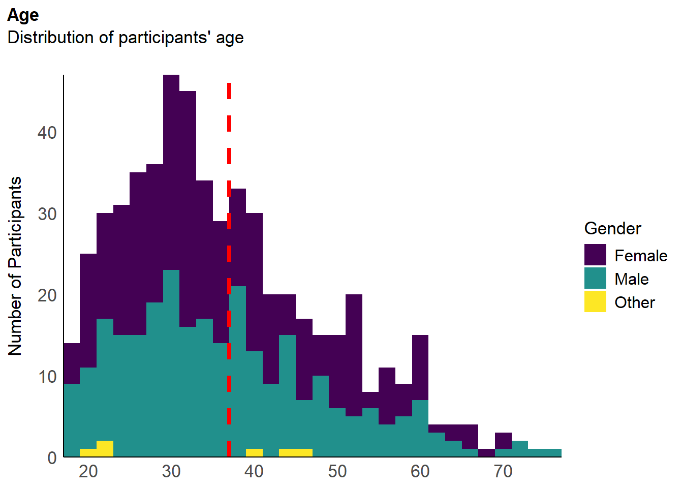

Code

# Did not add education disciplines 

p_edu <- df |>
  mutate (Student = ifelse(is.na(Student), FALSE, Student)) |>
  ggplot(aes(x = Education)) +
  geom_bar(aes(fill = Student)) +
  scale_y_continuous(expand = c(0, 0), breaks= scales::pretty_breaks()) +
  labs(title = "Education", y = "Number of Participants", subtitle = "Participants per achieved education level", fill = "Is currently a student") +
  theme_modern(axis.title.space = 15) +
  theme(
    plot.title = element_text(size = rel(1.2), face = "bold", hjust = 0),
    plot.subtitle = element_text(size = rel(1.2), vjust = 7),
    axis.text.y = element_text(size = rel(1.1)),
    axis.text.x = element_text(size = rel(0.5), angle = 45, hjust =1),
    axis.title.x = element_blank()
  )

p_edu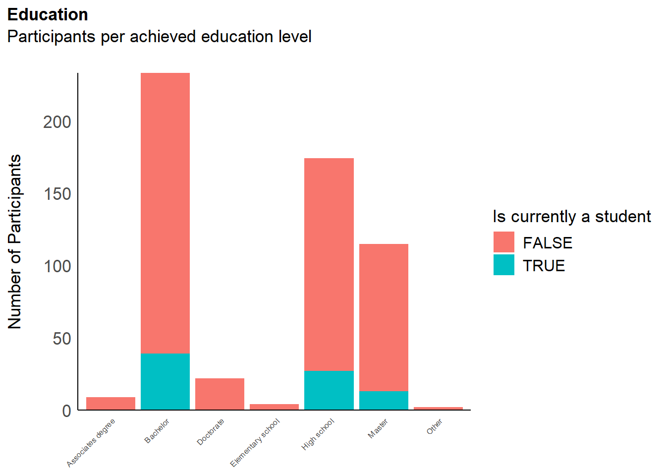

Code

p_eth <- df |>
  filter(!is.na(Ethnicity)) |> 
  ggplot(aes(x = "", fill = Ethnicity)) +
  geom_bar() +
  coord_polar("y") +
  theme_minimal() +
  theme(
    axis.text.x = element_blank(),
    axis.title.x = element_blank(),
    axis.text.y = element_blank(),
    axis.title.y = element_blank()
  )
    
p_eth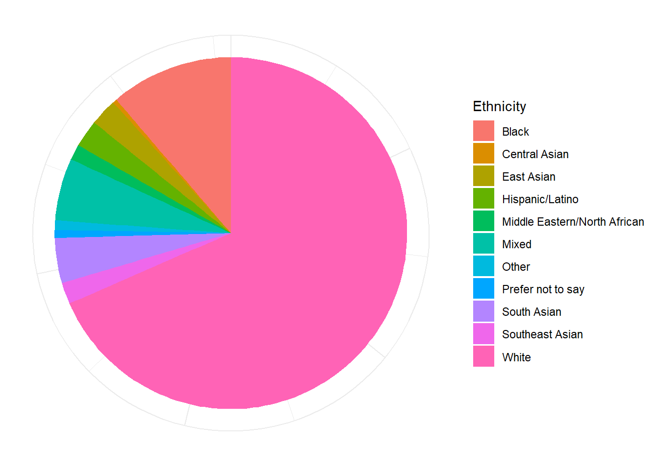

Code

p_map <- df |>
  mutate(Country = case_when(
    Country=="United States"~ "USA",
    Country=="United Kingdom" ~ "UK",
    TRUE ~ Country
  ))|>
  dplyr::select(region = Country) |>
  group_by(region) |>
  summarize(n = n()) |>
  right_join(map_data("world"), by = "region") |>
  # mutate(n = replace_na(n, 0)) |>
  ggplot(aes(long, lat, group = group)) +
  geom_polygon(aes(fill = n)) +
  scale_fill_gradientn(colors = c("#E66101", "#ca0020", "#cc66cc")) +
  labs(fill = "N") +
  theme_void() +
  labs(title = "Country of Residence", subtitle = "Number of participants by country")  +
  theme(
    plot.title = element_text(size = rel(1.2), face = "bold", hjust = 0),
    plot.subtitle = element_text(size = rel(1.2))
  )

p_map

Code

sort(table(df$Country)) |> 
  as.data.frame() |> 
  gt::gt()

Var1	Freq
Afghanistan	1
Albania	1
Canada	1
Ireland	17
Australia	27
United States	149
United Kingdom	357

Code

(p_age | p_edu) / p_map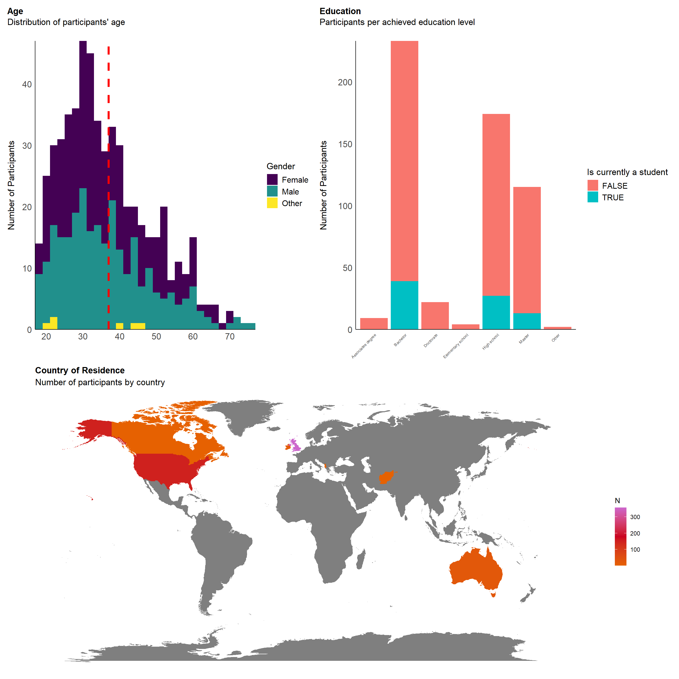

Save

Code

write.csv(df, "../data/data_participants.csv", row.names = FALSE)