Interoception Scale (Study 2) - Data Cleaning

Data Preparation

library(tidyverse)
library(easystats)
library(patchwork)
library(ggside)
library(ggdist)

df <- read.csv("../data/rawdata_participants.csv")

Recruitment History

Code

# Consecutive count of participants per day (as area)
df |>
  mutate(Date = as.Date(Experiment_StartDate, format = "%Y-%m-%d %H:%M:%S")) |> 
  summarize(N = n(), .by=c("Date", "Recruitment")) |> 
  complete(Date, Recruitment, fill = list(N = 0)) |> 
  mutate(N = cumsum(N), .by="Recruitment") |>
  ggplot(aes(x = Date, y = N)) +
  geom_area(aes(fill=Recruitment)) +
  scale_y_continuous(expand = c(0, 0)) +
  labs(
    title = "Recruitment History",
    x = "Date",
    y = "Total Number of Participants"
  ) +
  see::theme_modern()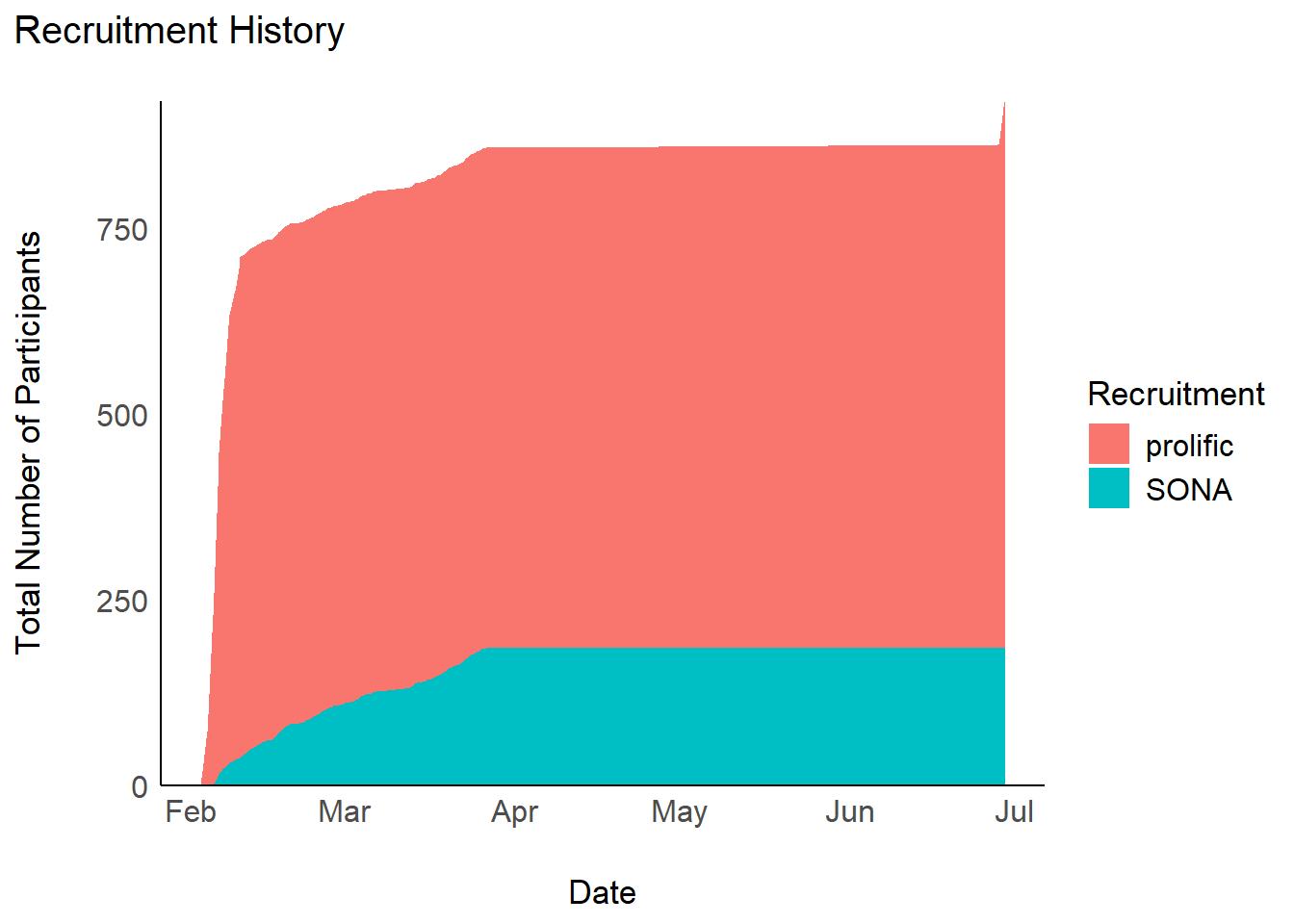

Code

# Table
summarize(df, N = n(), .by=c("Recruitment")) |> 
  arrange(desc(N)) |> 
  gt::gt() |> 
  gt::grand_summary_rows(columns = "N", fns = Total ~ sum(.)) |> 
  gt::opt_stylize(style = 2, color = "gray") |> 
  gt::tab_header("Number of participants per recruitment source")

Number of participants per recruitment source
	Recruitment	N
	prolific	736
	SONA	185
Total	—	921

Feedback

Experiment Enjoyment

Code

df |> 
  summarise(n = n(), .by=c("Experiment_Enjoyment")) |>
  filter(!is.na(Experiment_Enjoyment)) |> 
  mutate(n = n / sum(n),
         Experiment_Enjoyment = fct_rev(as.factor(Experiment_Enjoyment))) |>
  ggplot(aes(y = n, x = 1, fill = Experiment_Enjoyment)) +
  geom_bar(stat="identity", position="stack") +
  scale_fill_manual(values=c("green", "yellowgreen",  "yellow", "orange", "red")) +
  coord_flip() +
  scale_x_continuous(expand=c(0, 0))  +
  scale_y_continuous(labels = scales::percent)  +
  labs(title="Experiment Enjoyment",
       subtitle="Proportion of participants by condition") + 
  guides(fill = guide_legend(reverse=TRUE)) +
  theme_minimal() +
  theme(
    axis.title = element_blank(),
    axis.text.y = element_blank(),
    panel.grid.major.y = element_blank(),
    panel.grid.minor.y = element_blank(),
    legend.position = "top",
    legend.title = element_blank())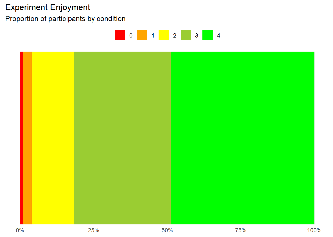

Comments

Code

data.frame(Comments = df$Experiment_Feedback) |> 
  filter(!tolower(Comments) %in% c(NA, "no", "none", "no thank you", "no not at all", "no thanks", "no comment", "nil", "n.a", "n/a", "na", "not really", "thank you", "nothing", "no not at the moment", "none for now", "thank you!", "thanks", "not really.")) |> 
  gt::gt() |> 
  gt::opt_stylize() |> 
  gt::opt_interactive(use_compact_mode = TRUE)

Exclusions

Code

outliers <- list()

Attention Checks

Code

dfchecks <- df |>
  dplyr::mutate(
    # "I can always accurately answer to the extreme left on this question to show that I am reading it"
    A1 = ifelse(MINT_AttentionCheck_1 == 0, 0, 1),
    # "I notice that I am being asked to respond all the way to the right"
    A2 = ifelse(MAIA_AttentionCheck_1 == 6, 0, 1),
    # "I can always accurately choose the lowest option"
    A3 = ifelse(IAS_AttentionCheck_1 == 1, 0, 1),
    # "Respond all the way to the right."
    A4 = ifelse(BodyAwareness_AttentionCheck_1 == 5, 0, 1),
    # "I am able to respond all the way to the left"
    A5 = ifelse(TAS_AttentionCheck_1 == 1, 0, 1),
    # "On the whole, I know I must press the highest option"
    A6 = ifelse(PI18_AttentionCheck_1 == 5, 0, 1),
    # "I feel that to show I'm being attentive I will press the lowest option"
    A7 = ifelse(CEFSA_AttentionCheck_1 == 0, 0, 1),
    .keep = "none"
  ) 
dfchecks$Total <- rowSums(dfchecks)


dfchecks |>
  mutate(Total = as.factor(paste0(Total, "/8"))) |> 
  ggplot(aes(x = Total)) +
  geom_bar(aes(fill = Total)) +
  scale_fill_viridis_d(guide = "none") +
  labs(title = "Failed Attention Checks", y = "Number of Participants", subtitle = "Number of failed attention checks per participant") +
  theme_modern(axis.title.space = 15) +
  theme(
    plot.title = element_text(size = rel(1.2), face = "bold", hjust = 0),
    plot.subtitle = element_text(size = rel(1.2), vjust = 7),
    axis.title.x = element_blank(),
  )

Code

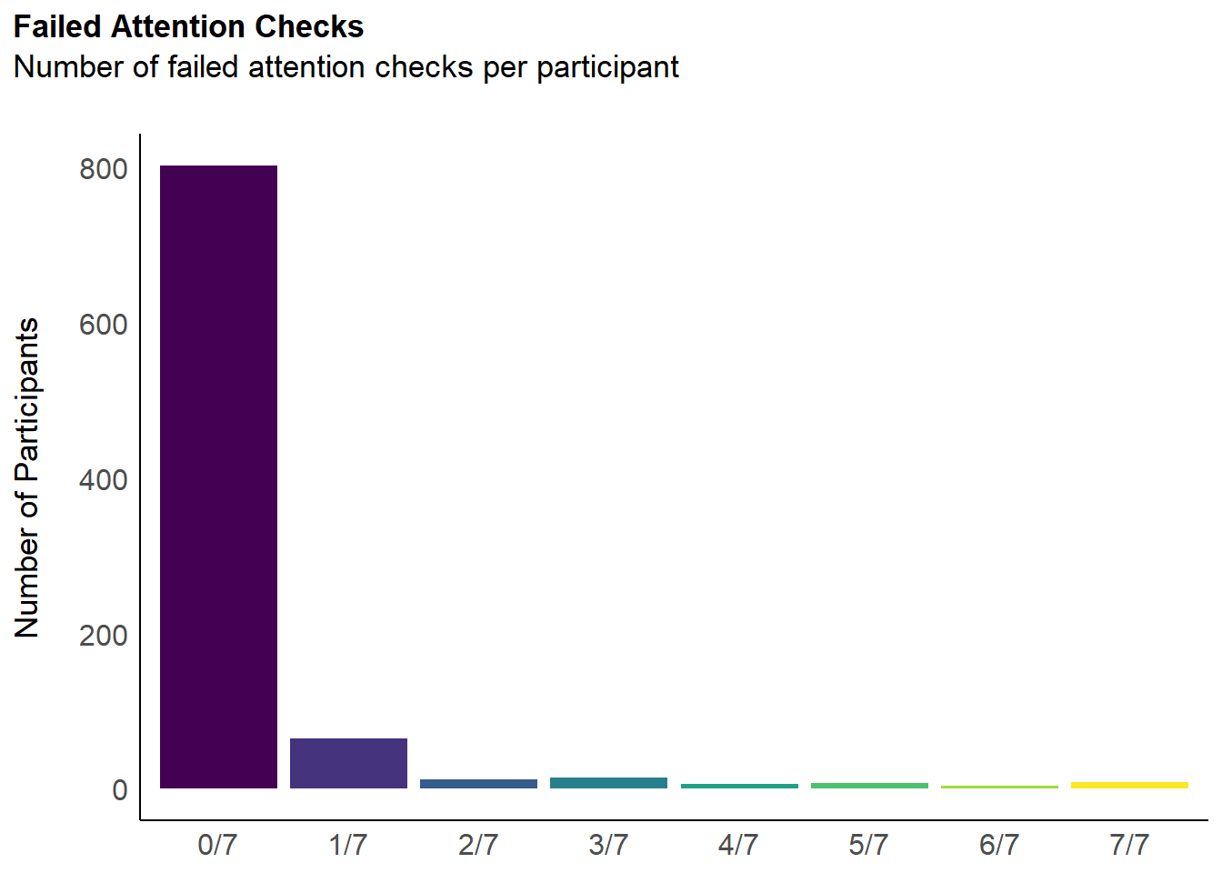
outliers$attentionchecks <- df$Participant[dfchecks$Total >= 1]

We removed 118 (12.81%) participants for having failed at least 1 attention check (out of 8).

Experiment Duration

Code

dfchecks$Duration <- df$Experiment_Duration
dfchecks$Outlier <- ifelse(dfchecks$Total >= 1, 1, 0)
dfchecks <- filter(dfchecks, Duration < 45)

m <- mgcv::gam(Outlier ~ s(Duration), data = dfchecks, family = "binomial")

estimate_relation(m, length=50) |> 
  ggplot(aes(x = Duration, y = Predicted)) +
  geom_ribbon(aes(ymin = CI_low, ymax = CI_high), alpha = 0.2) +
  geom_line() +
  geom_vline(xintercept=10, linetype="dashed", color="red") +
  theme_minimal() +
  ggside::geom_xsidedensity(data=mutate(dfchecks, 
                                        Outlier=ifelse(Outlier==1, "Failed attention check", "Valid")), 
                            aes(fill=Outlier), alpha=0.3) +
  ggside::theme_ggside_void() +
  labs(title = "Experiment Duration",
       subtitle = "Predicted probability of failing attention checks by duration",
       x = "Experiment Duration (minutes)",
       y = "Probability of failing attention checks")

Warning: `is.ggproto()` was deprecated in ggplot2 3.5.2.
ℹ Please use `is_ggproto()` instead.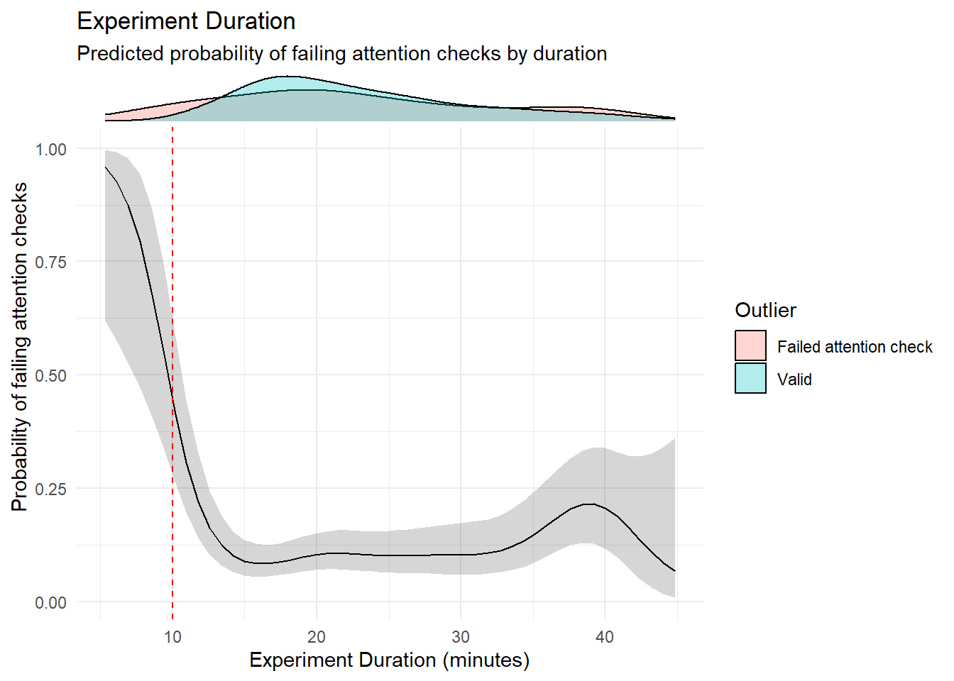

Code

outliers$duration <- as.character(df[df$Experiment_Duration < 10, "Participant"])
outliers$duration <- outliers$duration[!outliers$duration %in% outliers$attentionchecks]

We removed 2 (0.22%) participants for having completed the experiment in less than 5 minutes.

Multivariate Distance

Code

# Compute distance
dfoutlier <- performance::check_outliers(select(df, contains("MAIA_")), 
                                         method=c("optics"),
                                         threshold=list(optics=2.5, optics_xi=0.01)) |> 
  as.data.frame() |> 
  mutate(Participant = fct_reorder(df$Participant, Distance_OPTICS),
         Outlier_AttentionCheck = ifelse(Participant %in% outliers$attentionchecks, 1, 0),
         Outlier_Duration = ifelse(Participant %in% outliers$duration, 1, 0),
         Outlier = ifelse(Outlier_AttentionCheck == 1, "Failed Attention Checks", "Passed"),
         Outlier = ifelse(Outlier == "Passed" & Outlier_Duration == 1, "Duration", Outlier))


outliers$distance <- as.character(dfoutlier[dfoutlier$Distance_OPTICS < 3.3, "Participant"])
outliers$distance <- outliers$distance[!outliers$distance %in% c(outliers$attentionchecks, outliers$duration)]


p1 <- dfoutlier |> 
  ggplot(aes(x=Participant, y=Distance_OPTICS)) +
  geom_bar(aes(fill=Outlier), stat="identity") +
  geom_hline(yintercept = 3.3, linetype="dashed", color="red") +
  labs(fill = "Status") +
  scale_fill_manual(values=c("Duration" = "purple", "Failed Attention Checks"="red", "Passed"="grey")) +
  theme_minimal() +
  theme(axis.text.x = element_blank(),
        panel.grid.major.x = element_blank())

m <- mgcv::gam(Outlier_AttentionCheck ~ s(Distance_OPTICS), data = dfoutlier, family = "binomial")
# parameters::parameters(m)

p2 <- estimate_relation(m, length=30) |> 
  ggplot(aes(x=Distance_OPTICS, y=Predicted)) +
  geom_ribbon(aes(ymin=CI_low, ymax=CI_high), alpha=0.2) +
  geom_line() +
  geom_vline(xintercept=3.3, linetype="dashed", color="red") +
  geom_hline(yintercept=1/3, linetype="dashed", color="black") +
  theme_minimal() 

p1 | p2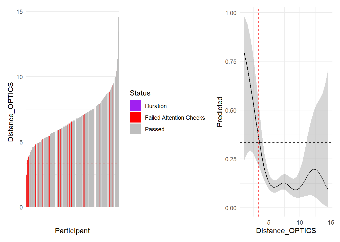

We removed 4 (0.43%) participants based on multivariate distance.

df <- filter(df, !Participant %in% c(outliers$attentionchecks, outliers$duration, outliers$distance))

Dimension Computation

Code

compute_and_remove <- function(df, name="BodyAwareness", pattern=name, method="mean") {
  items <- select(df, starts_with(pattern), -contains("AttentionCheck"))
  df <- df[!names(df) %in% names(items)]
  if(method == "mean") {
    df[[name]] <- rowMeans(items, na.rm=TRUE)
  } else {
    df[[name]] <- rowSums(items, na.rm=TRUE)
  }
  df
}

df <- compute_and_remove(df, name="IAS", method="sum")

df <- compute_and_remove(df, name="BPQ", pattern="BodyAwareness", method="mean")


df[grepl("^MAIA_.*_R$", names(df))] <- 6 - df[grepl("^MAIA_.*_R$", names(df))]  # Reverse
df <- compute_and_remove(df, name="MAIA_AttentionRegulation", method="mean")
df <- compute_and_remove(df, name="MAIA_BodyListening", method="mean")
df <- compute_and_remove(df, name="MAIA_EmotionalAwareness", method="mean")
df <- compute_and_remove(df, name="MAIA_NotDistracting", method="mean")
df <- compute_and_remove(df, name="MAIA_Noticing", method="mean")
df <- compute_and_remove(df, name="MAIA_NotWorrying", method="mean")
df <- compute_and_remove(df, name="MAIA_SelfRegulation", method="mean")
df <- compute_and_remove(df, name="MAIA_Trusting", method="mean")

df <- compute_and_remove(df, name="PHQ4_Anxiety", method="sum")
df <- compute_and_remove(df, name="PHQ4_Depression", method="sum")

# TODO: check if any reversed items in the following questionnaires
df <- compute_and_remove(df, name="TAS_EOT", method="mean")
df <- compute_and_remove(df, name="TAS_DDF", method="mean")
df <- compute_and_remove(df, name="TAS_DIF", method="mean")

df <- compute_and_remove(df, name="ERS_Arousal", method="mean")
df <- compute_and_remove(df, name="ERS_Sensitivity", method="mean")
df <- compute_and_remove(df, name="ERS_Persistence", method="mean")

df <- compute_and_remove(df, name="CERQ_Acceptance", method="mean")
df <- compute_and_remove(df, name="CERQ_PositiveRefocusing", method="mean")
df <- compute_and_remove(df, name="CERQ_PositiveReappraisal", method="mean")
df <- compute_and_remove(df, name="CERQ_SelfBlame", method="mean")
df <- compute_and_remove(df, name="CERQ_OtherBlame", method="mean")
df <- compute_and_remove(df, name="CERQ_Rumination", method="mean")
df <- compute_and_remove(df, name="CERQ_Catastrophizing", method="mean")
df <- compute_and_remove(df, name="CERQ_RefocusPlanning", method="mean")
df <- compute_and_remove(df, name="CERQ_Perspective", method="mean")

df <- compute_and_remove(df, name="CEFSA_Body", method="mean")
df <- compute_and_remove(df, name="CEFSA_Agency", method="mean")
df <- compute_and_remove(df, name="CEFSA_Emotion", method="mean")
df <- compute_and_remove(df, name="CEFSA_Familiarity", method="mean")
df <- compute_and_remove(df, name="CEFSA_Connection", method="mean")
df <- compute_and_remove(df, name="CEFSA_Reality", method="mean")
df <- compute_and_remove(df, name="CEFSA_Self", method="mean")

df[grepl("^PI18.*_R$", names(df))] <- 6 - df[grepl("^PI18.*_R$", names(df))]  # Reverse
df$PI_Alive <- rowMeans(df[grepl("^PI18.*A_", names(df))], na.rm=TRUE)
df <- compute_and_remove(df, name="PI_Safe", pattern="PI18_GS", method="mean")
df <- compute_and_remove(df, name="PI_Enticing", pattern="PI18_GE", method="mean")
df$PI_Good <- rowMeans(select(df, PI_Safe, PI_Enticing), na.rm=TRUE)
df <- select(df, -starts_with("PI18_"))

Final Sample

We removed 60 participants with missing data for the MINT due to a technical error.

df <- filter(df, !is.na(df$MINT_Awareness_RelA_29))

The final sample includes 737 participants (Mean age = 36.8, SD = 14.9, range: [17, 87]; Gender: 57.3% women, 41.1% men, 1.63% non-binary; Education: Bachelor, 31.48%; Doctorate, 2.44%; Elementary school, 0.41%; High school, 51.70%; Master, 13.98%; Country: 75.17% United Kingdom, 24.83% other).

Code

p_age <- df |>
  ggplot(aes(x = Age, fill = Gender)) + 
  geom_histogram(data=df, aes(x = Age, fill=Gender), binwidth = 2) +
  geom_vline(xintercept = mean(df$Age), color = "red", linewidth=1.5, linetype="dashed") +
  scale_fill_viridis_d() +
  scale_x_continuous(expand = c(0, 0), breaks = seq(20, max(df$Age), by = 10 )) +
  scale_y_continuous(expand = c(0, 0)) +
  labs(title = "Age", y = "Number of Participants", color = NULL, subtitle = "Distribution of participants' age") +
  theme_modern(axis.title.space = 10) +
  theme(
    plot.title = element_text(size = rel(1.2), face = "bold", hjust = 0),
    plot.subtitle = element_text(size = rel(1.2), vjust = 7),
    axis.text.y = element_text(size = rel(1.1)),
    axis.text.x = element_text(size = rel(1.1)),
    axis.title.x = element_blank()
  )

p_age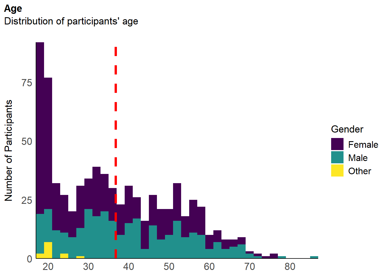

Code

p_edu <- df |>
  mutate(Student = ifelse(is.na(Student), FALSE, Student),
         Education = fct_relevel(Education, "High school", "Bachelor", "Master", "Doctorate")) |>
  ggplot(aes(x = Education)) +
  geom_bar(aes(fill = Student)) +
  scale_y_continuous(expand = c(0, 0), breaks= scales::pretty_breaks()) +
  labs(title = "Education", y = "Number of Participants", subtitle = "Participants per achieved education level", fill = "Is currently a student") +
  theme_modern(axis.title.space = 15) +
  theme(
    plot.title = element_text(size = rel(1.2), face = "bold", hjust = 0),
    plot.subtitle = element_text(size = rel(1.2), vjust = 7),
    axis.text.y = element_text(size = rel(1.1)),
    axis.text.x = element_text(size = rel(0.5), angle = 45, hjust =1),
    axis.title.x = element_blank()
  )

p_edu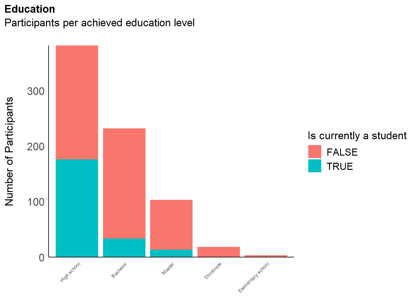

Code

p_eth <- df |>
  filter(!is.na(Ethnicity)) |> 
  ggplot(aes(x = "", fill = Ethnicity)) +
  geom_bar() +
  coord_polar("y") +
  theme_minimal() +
  theme(
    axis.text.x = element_blank(),
    axis.title.x = element_blank(),
    axis.text.y = element_blank(),
    axis.title.y = element_blank()
  )
    
p_eth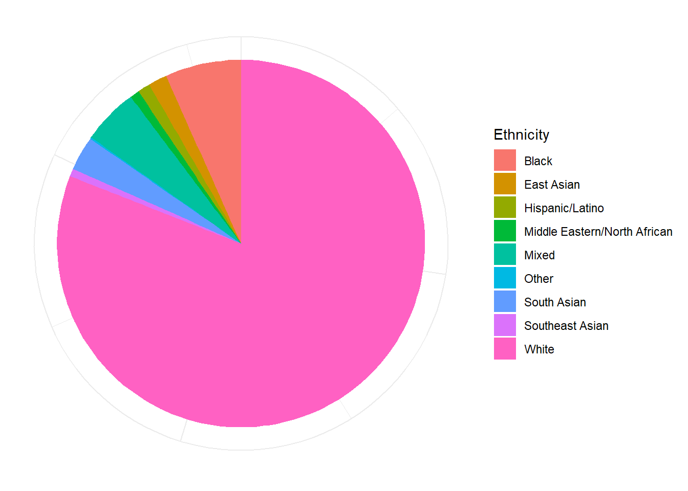

Code

p_map <- df |>
  mutate(Country = case_when(
    Country=="United States"~ "USA",
    Country=="United Kingdom" ~ "UK",
    TRUE ~ Country
  ))|>
  dplyr::select(region = Country) |>
  group_by(region) |>
  summarize(n = n()) |>
  right_join(map_data("world"), by = "region") |>
  # mutate(n = replace_na(n, 0)) |>
  ggplot(aes(long, lat, group = group)) +
  geom_polygon(aes(fill = n)) +
  scale_fill_gradientn(colors = c("#E66101", "#ca0020", "#cc66cc")) +
  labs(fill = "N") +
  theme_void() +
  labs(title = "Country of Residence", subtitle = "Number of participants by country")  +
  theme(
    plot.title = element_text(size = rel(1.2), face = "bold", hjust = 0),
    plot.subtitle = element_text(size = rel(1.2))
  )

p_map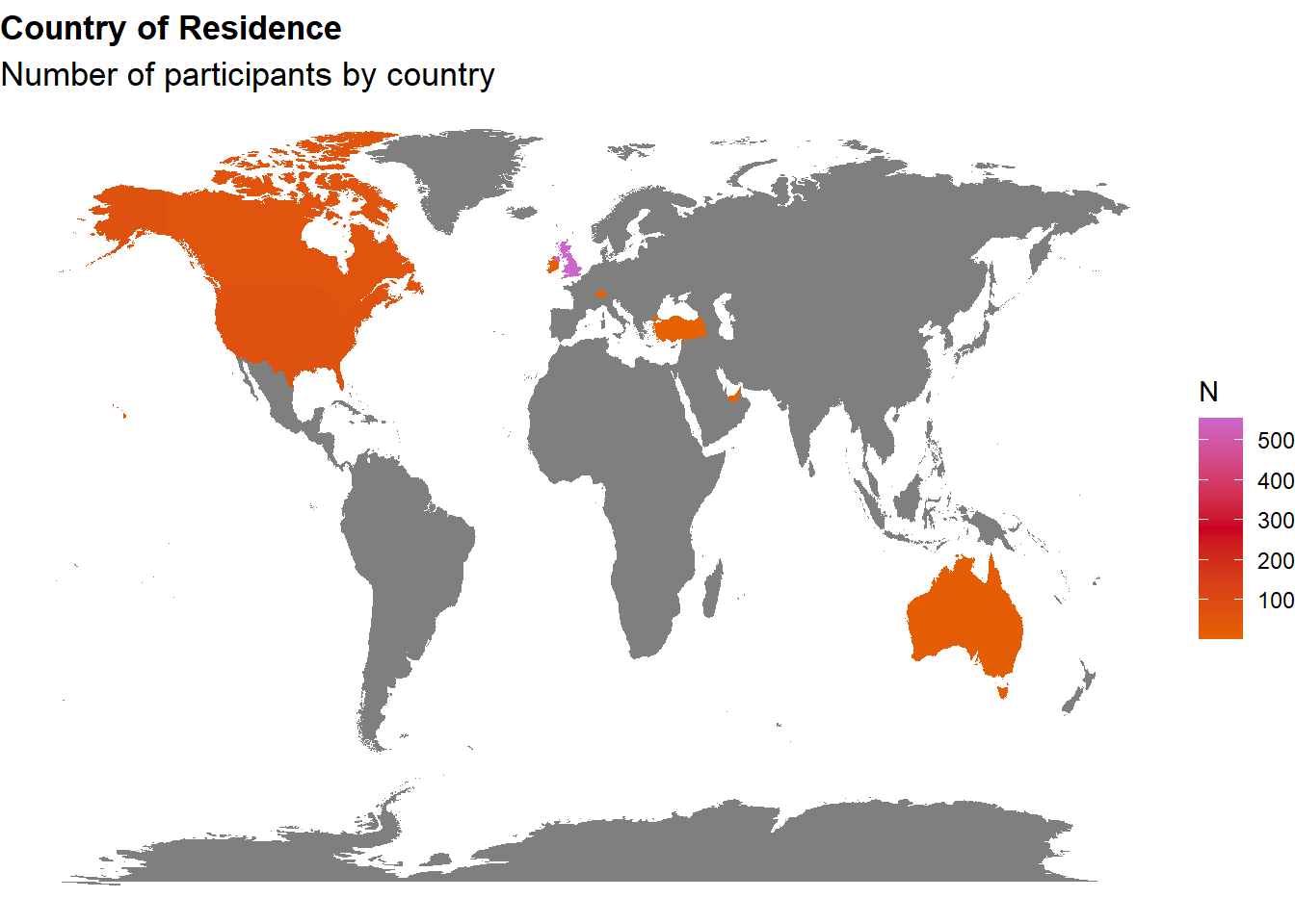

Code

sort(table(df$Country)) |> 
  as.data.frame() |>
  rename(Country = Var1) |> 
  arrange(desc(Freq)) |> 
  gt::gt()

Country	Freq
United Kingdom	554
United States	72
Canada	58
Ireland	19
Australia	17
Switzerland	1
Turkey	1
United Arab Emirates	1

Code

p_bmi <- df |> 
  filter(!is.na(BMI), Gender != "Other") |> 
  ggplot(aes(x=BMI)) +
  annotate("rect", xmin=10, xmax=18.5, ymin=0, ymax=Inf, fill="red", alpha=0.1) +
  annotate("rect", xmin=18.5, xmax=25, ymin=0, ymax=Inf, fill="green", alpha=0.25) +
  annotate("rect", xmin=25, xmax=30, ymin=0, ymax=Inf, fill="yellow", alpha=0.25) +
  annotate("rect", xmin=30, xmax=40, ymin=0, ymax=Inf, fill="orange", alpha=0.25) +
  annotate("rect", xmin=40, xmax=Inf, ymin=0, ymax=Inf, fill="red", alpha=0.1) +
  geom_density(aes(color=Gender, fill=Gender), alpha=0.5, linewidth=2) +
  labs(title = "BMI distribution") +
  scale_fill_manual(values = c("Male"= "#64B5F6", "Female"= "#F06292", "Other"="orange", "Missing"="brown")) +
  scale_color_manual(values = c("Male"= "#64B5F6", "Female"= "#F06292", "Other"="orange", "Missing"="brown")) +
  theme_minimal() +
  theme(axis.title.y = element_blank(),
        axis.text.y = element_blank())

p_bmi_a <- df |> 
  filter(!is.na(BMI), Gender != "Other") |> 
  ggplot(aes(x=Age, y=BMI, color=Gender)) +
  geom_point(size=3, alpha=0.5) +
  geom_smooth(aes(fill=Gender), alpha=0.3, method = 'loess', formula = 'y ~ x') +
  scale_fill_manual(values = c("Male"= "#64B5F6", "Female"= "#F06292", "Other"="orange", "Missing"="brown")) +
  scale_color_manual(values = c("Male"= "#64B5F6", "Female"= "#F06292", "Other"="orange", "Missing"="brown")) +
  theme_minimal() +
  theme(legend.position = "none")

p_bmi_b <- df |> 
  filter(!is.na(BMI), Gender != "Other") |> 
  ggplot(aes(x=Physical_Active, y=BMI)) +
  geom_jitter(aes(color=Gender), width=0.1, size=3, alpha=0.5) +
  geom_smooth(aes(fill=Gender, color=Gender), alpha=0.3, method = 'lm', formula = 'y ~ x') +
  labs(x = "Physically Active", y = "") +
  scale_x_continuous(breaks=0:7) +
  scale_fill_manual(values = c("Male"= "#64B5F6", "Female"= "#F06292", "Other"="orange", "Missing"="brown")) +
  scale_color_manual(values = c("Male"= "#64B5F6", "Female"= "#F06292", "Other"="orange", "Missing"="brown")) +
  theme_minimal() +
  theme(legend.position = "none",
        panel.grid.minor.x = element_blank()) +
  ggside::geom_xsidehistogram(aes(fill=Gender), bins = 30, position="dodge") +
  ggside::theme_ggside_void()

df$Physical_Workout[df$Physical_Workout > 25] <- NA

p_bmi_c <- df |> 
  filter(!is.na(BMI) & !is.na(Physical_Workout), Gender != "Other") |> 
  ggplot(aes(x=Physical_Workout, y=BMI)) +
  geom_point(aes(color=Gender), size=3, alpha=0.5) +
  geom_smooth(aes(fill=Gender, color=Gender), alpha=0.3, method = 'lm', formula = 'y ~ x') +
  labs(x = "Hours of Active Workout", y = "") +
  scale_fill_manual(values = c("Male"= "#64B5F6", "Female"= "#F06292", "Other"="orange", "Missing"="brown")) +
  scale_color_manual(values = c("Male"= "#64B5F6", "Female"= "#F06292", "Other"="orange", "Missing"="brown")) +
  theme_minimal() +
  theme(legend.position = "none") +
  ggside::geom_xsidehistogram(aes(fill=Gender), bins = 30, position="dodge") +
  ggside::theme_ggside_void()

p_bmi / (p_bmi_a | p_bmi_b | p_bmi_c)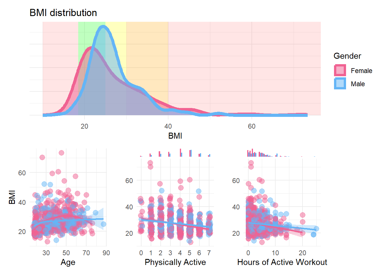

Code

df$Disorders_Psychiatric_Mood <- ifelse(str_detect(df$Disorders_Psychiatric, "MDD|GAD|Bipolar"), TRUE, FALSE)
df$Disorders_Psychiatric_MoodTreatment <- ifelse(
  df$Disorders_Psychiatric_Mood & !is.na(df$Disorders_PsychiatricTreatment) & str_detect(df$Disorders_PsychiatricTreatment, "Mood|Antidepressant|Anxiolytic|Psychotherapy"), TRUE, FALSE)

df$Disorders_Psychiatric_Anxiety <- ifelse(str_detect(df$Disorders_Psychiatric, "Panic|GAD|Social Phobia|Phobia"), TRUE, FALSE)
df$Disorders_Psychiatric_AnxietyTreatment <- ifelse(
  df$Disorders_Psychiatric_Anxiety & !is.na(df$Disorders_PsychiatricTreatment) & str_detect(df$Disorders_PsychiatricTreatment, "Anxiolytic|Psychotherapy|Mindfulness"), TRUE, FALSE)

df$Disorders_Psychiatric_Eating <- ifelse(str_detect(df$Disorders_Psychiatric, "Eating"), TRUE, FALSE)
df$Disorders_Psychiatric_Addiction <- ifelse(str_detect(df$Disorders_Psychiatric, "Addiction"), TRUE, FALSE)
df$Disorders_Psychiatric_Borderline <- ifelse(str_detect(df$Disorders_Psychiatric, "BPD"), TRUE, FALSE)

df$Disorders_Psychiatric_Autism <- ifelse(str_detect(df$Disorders_Psychiatric, "ASD"), TRUE, FALSE)
df$Disorders_Psychiatric_ADHD <- ifelse(str_detect(df$Disorders_Psychiatric, "ADHD"), TRUE, FALSE)


# df$Disorders_Psychiatric_Other <- ifelse(str_detect(df$Disorders_Psychiatric, "MDD|GAD|Bipolar"), TRUE, FALSE)

select(df, Participant, Gender, 
             Disorders_Psychiatric_Mood, Disorders_Psychiatric_MoodTreatment,
             Disorders_Psychiatric_Anxiety, Disorders_Psychiatric_AnxietyTreatment,
             Disorders_Psychiatric_Eating, Disorders_Psychiatric_Addiction, Disorders_Psychiatric_Borderline,
             Disorders_Psychiatric_Autism, Disorders_Psychiatric_ADHD) |> 
  pivot_longer(cols = starts_with("Disorders_"), names_to = "Disorder", values_to = "Value") |> 
  mutate(Disorder = str_remove_all(Disorder, fixed("Disorders_Psychiatric_")),
         Disorder = str_replace(Disorder, "MoodTreatment", "Mood Disorder (with treatment)"),
         Disorder = str_replace(Disorder, "AnxietyTreatment", "Anxiety (with treatment)"),
         Disorder = str_replace(Disorder, "Mood$", "Mood Disorder")) |> 
  summarize(N = sum(Value) / nrow(df), .by=c("Gender", "Disorder")) |> 
  mutate(N_tot = sum(N), .by="Disorder") |>
  mutate(Disorder = fct_reorder(Disorder, desc(N_tot)),
         Treatment = ifelse(str_detect(Disorder,  "Treatment"), "With treatment", "Without treatment")) |>
  ggplot(aes(x = Disorder, y = N, fill=Gender)) +
  geom_bar(stat = "identity") +
  scale_fill_manual(values = c("Male"= "#64B5F6", "Female"= "#F06292", "Other"="orange", "Missing"="brown")) +
  scale_y_continuous(expand = c(0, 0), labels=scales::percent) +
  labs(title = "Mood Disorders", y = "Number of Participants", subtitle = "Participants per self-declared mood disorder", x="Type") +
  theme_minimal() +
  theme(axis.text.x = element_text(angle = 45, hjust = 1))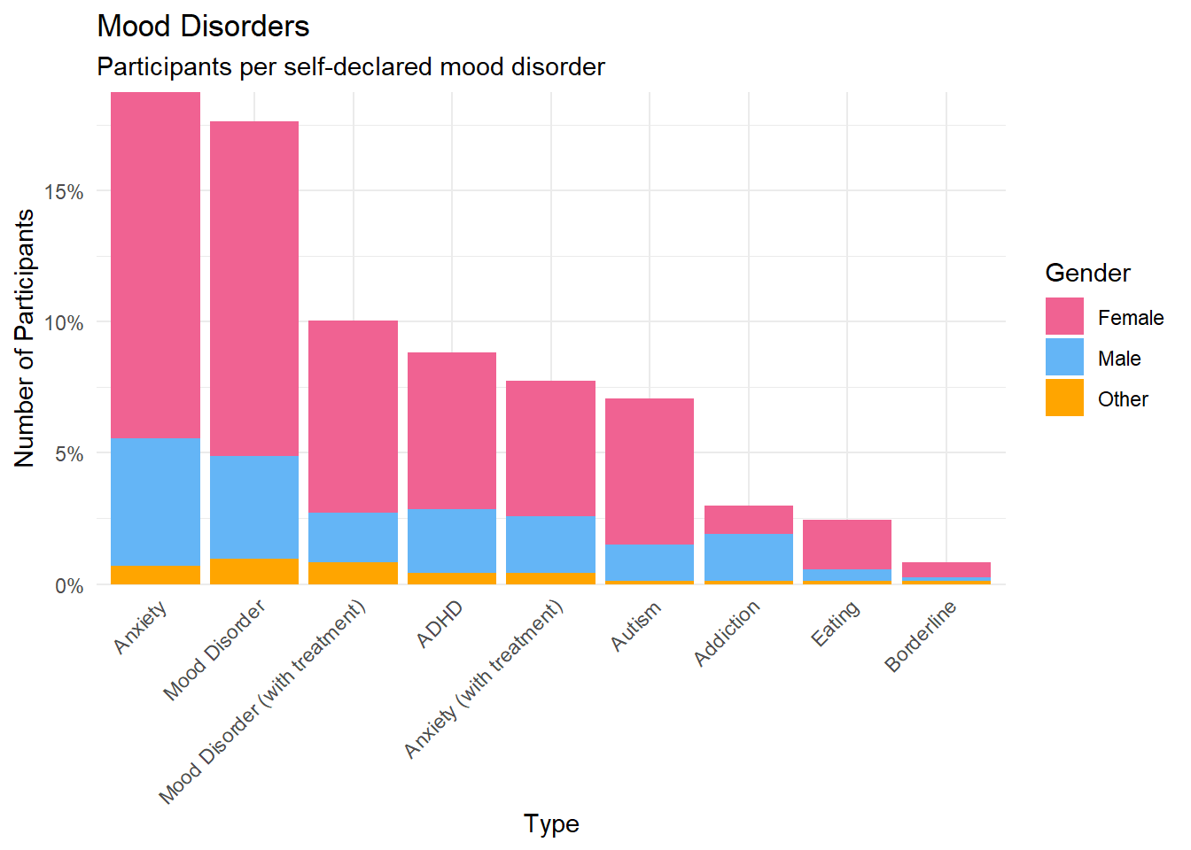

Code

somatic <- data.frame(
  Hypermobility = ifelse(str_detect(df$Disorders_Somatic, "Hypermobility Syndrome"), TRUE, FALSE),
  Fibromyalgia = ifelse(str_detect(df$Disorders_Somatic, "Fibromyalgia"), TRUE, FALSE),
  ChronicFatigue = ifelse(str_detect(df$Disorders_Somatic, "Chronic Fatigue Syndrome"), TRUE, FALSE),
  ChronicPain = ifelse(str_detect(df$Disorders_Somatic, "Chronic Pain Syndrome"), TRUE, FALSE),
  BackPain = ifelse(str_detect(df$Disorders_Somatic, "Back Pain"), TRUE, FALSE),
  MuscleTension = ifelse(str_detect(df$Disorders_Somatic, "Muscle Tension"), TRUE, FALSE),
  SkinRashes = ifelse(str_detect(df$Disorders_Somatic, "Skin Rashes"), TRUE, FALSE),
  Eczema = ifelse(str_detect(df$Disorders_Somatic, "Eczema"), TRUE, FALSE),
  Psoriasis = ifelse(str_detect(df$Disorders_Somatic, "Psoriasis"), TRUE, FALSE),
   # Dermatological = ifelse(str_detect(df$Disorders_Somatic, "Other Dermatological"), TRUE, FALSE),
  # Musculoskeletal = ifelse(str_detect(df$Disorders_Somatic, "Other Musculoskeletal"), TRUE, FALSE),
  Sjogrens = ifelse(str_detect(df$Disorders_Somatic, "Sjogren"), TRUE, FALSE),
  ChestPain = ifelse(str_detect(df$Disorders_Somatic, "Chest Pain"), TRUE, FALSE),
  Arrhythmia = ifelse(str_detect(df$Disorders_Somatic, "Cardiac Arrhythmia"), TRUE, FALSE),
  Hypertension = ifelse(str_detect(df$Disorders_Somatic, "Hypertension"), TRUE, FALSE),
  Hypotension = ifelse(str_detect(df$Disorders_Somatic, "Hypotension"), TRUE, FALSE),
  IBS = ifelse(str_detect(df$Disorders_Somatic, "IBS"), TRUE, FALSE),
  GERD = ifelse(str_detect(df$Disorders_Somatic, "GERD"), TRUE, FALSE),
  Crohn = ifelse(str_detect(df$Disorders_Somatic, "Crohn"), TRUE, FALSE),
  UlcerativeColitis = ifelse(str_detect(df$Disorders_Somatic, "Ulcerative Colitis"), TRUE, FALSE),
  Celiac = ifelse(str_detect(df$Disorders_Somatic, "Celiac Disease"), TRUE, FALSE),
  Gluten = ifelse(str_detect(df$Disorders_Somatic, "Gluten"), TRUE, FALSE),
  Lactose = ifelse(str_detect(df$Disorders_Somatic, "Lactose"), TRUE, FALSE),
  ShortBreath = ifelse(str_detect(df$Disorders_Somatic, "Shortness of Breath"), TRUE, FALSE),
  Asthma = ifelse(str_detect(df$Disorders_Somatic, "Asthma"), TRUE, FALSE),
  COPD = ifelse(str_detect(df$Disorders_Somatic, "COPD"), TRUE, FALSE),
  SleepApnea = ifelse(str_detect(df$Disorders_Somatic, "Sleep Apnea"), TRUE, FALSE),
  Bronchitis = ifelse(str_detect(df$Disorders_Somatic, "Chronic Bronchitis"), TRUE, FALSE),
  Nausea = ifelse(str_detect(df$Disorders_Somatic, "Nausea/Vomiting"), TRUE, FALSE),
  Dizziness = ifelse(str_detect(df$Disorders_Somatic, "Dizziness/Lightheadedness"), TRUE, FALSE),
  Migraine = ifelse(str_detect(df$Disorders_Somatic, "Migraine"), TRUE, FALSE),
  Neuropathy = ifelse(str_detect(df$Disorders_Somatic, "Neuropathy"), TRUE, FALSE),
  Epilepsy = ifelse(str_detect(df$Disorders_Somatic, "Epilepsy"), TRUE, FALSE),
  MS = ifelse(str_detect(df$Disorders_Somatic, "Multiple Sclerosis"), TRUE, FALSE),
  FrequentUrination = ifelse(str_detect(df$Disorders_Somatic, "Frequent Urination"), TRUE, FALSE),
  Endometriosis = ifelse(str_detect(df$Disorders_Somatic, "Endometriosis"), TRUE, FALSE),
  Cystitis = ifelse(str_detect(df$Disorders_Somatic, "Interstitial Cystitis"), TRUE, FALSE),
  PelvicPain = ifelse(str_detect(df$Disorders_Somatic, "Chronic Pelvic Pain Syndrome"), TRUE, FALSE)
)


somatic |> 
  select(where(~n_distinct(.) > 1)) |> 
  correlation::correlation(redundant = TRUE, p_adjust="none") |>
  correlation::cor_sort() |> 
  mutate(label = ifelse(p < .001, "*", ""),
         label = ifelse(r == 1, "", label)) |> 
  ggplot(aes(x=Parameter1, y=Parameter2, fill=r)) +
  geom_tile() +
  geom_text(aes(label=label), size=3) +
  scale_fill_gradient2(low="blue", high="red", mid="white", midpoint=0) +
  labs(title = "Co-occurence Matrix of Somatic Disorders") +
  theme_minimal()  +
  theme(axis.text.x = element_text(angle=45, hjust=1),
        axis.title = element_blank())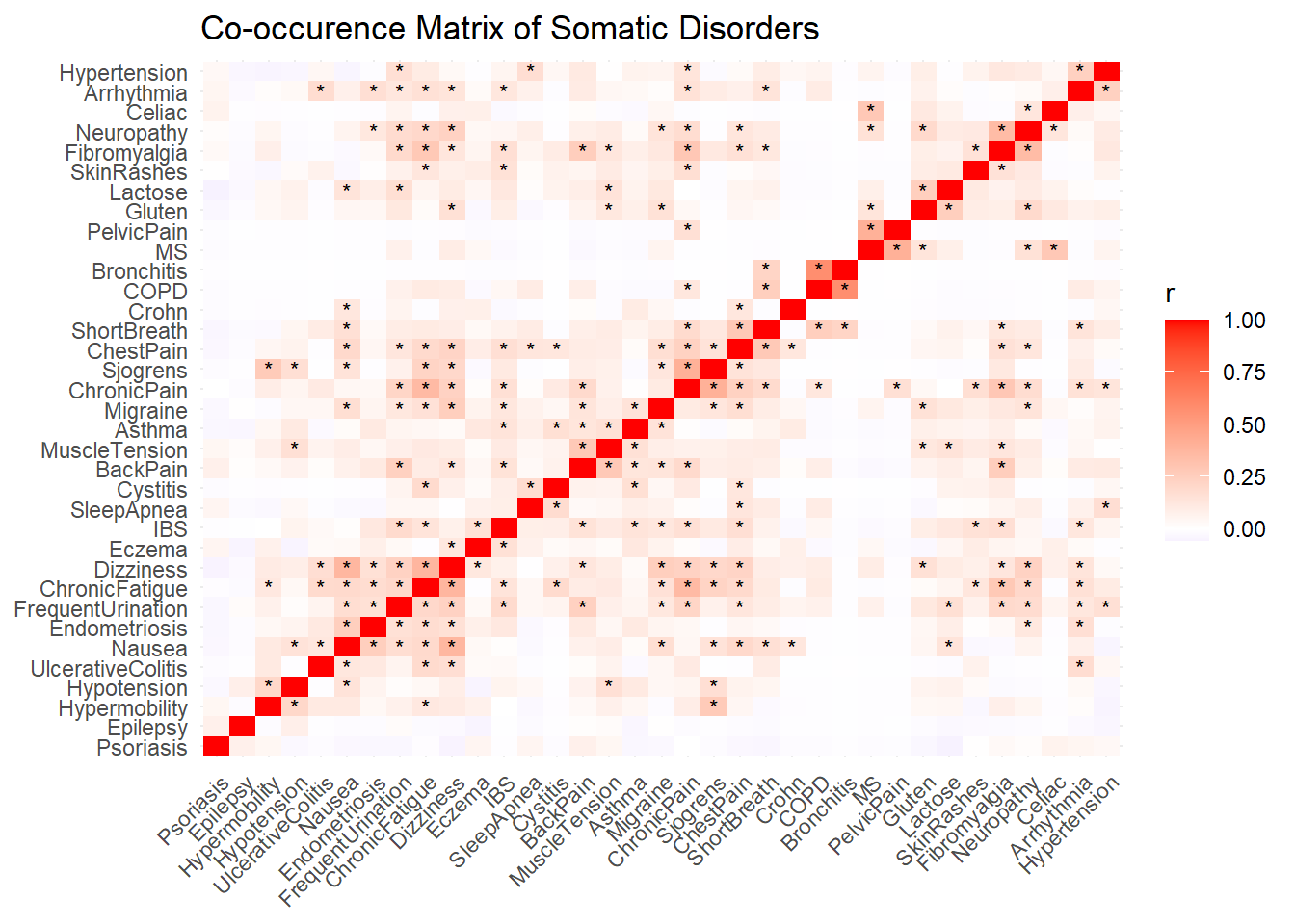

Code

# pca <- as.data.frame(prcomp(somatic)$rotation[, 1:5])
# pca$PC <- colnames(pca)[max.col(pca, ties.method='first')]
# 
# pca |> 
#   rownames_to_column(var="Disorder") |> 
#   pivot_longer(-c(Disorder, PC)) |> 
#   filter(PC == name) |> 
#   arrange(name, desc(value)) |> 
#   ggplot(aes(x=value, y=Disorder, fill=name)) +
#   geom_bar(stat = "identity") +
#   facet_wrap(~name, scale="free_y")

Code

# somatic |> 
#   select(where(~n_distinct(.) > 1)) |> 
#   EGAnet::bootEGA(
#     corr="pearson",
#     EGA.type = "EGA.fit",
#     model = "glasso", 
#     algorithm = "leiden",
#     seed=42)

To facilitate mechanistic interpretation and reduce redundancy, self-reported somatic symptoms were grouped into four non-overlapping clusters based on shared physiological pathways and known etiological mechanisms. The Afferent Sensitivity cluster included conditions associated with heightened interoceptive awareness and neurogenic excitability, such as migraine, neuropathy, dizziness, nausea, muscle tension, epilepsy, and frequent urination. The Central Sensitization cluster comprised syndromes characterized by chronic pain and fatigue, likely reflecting central amplification of sensory signals and HPA-axis dysregulation; this included fibromyalgia, chronic fatigue syndrome, chronic pain, back pain, pelvic pain, endometriosis, irritable bowel syndrome (IBS), and interstitial cystitis. The Autonomic Dysfunction cluster captured disorders linked to dysregulation of the autonomic and cardiopulmonary systems, including joint hypermobility, cardiac arrhythmia, chest pain, shortness of breath, hypo-/hypertension, sleep apnea, chronic obstructive pulmonary disease (COPD), and chronic bronchitis. Finally, the Immune-Inflammatory cluster encompassed conditions associated with immune dysregulation, barrier dysfunction, and gut-brain axis disturbance, such as eczema, psoriasis, skin rashes, asthma, celiac disease, gluten and lactose sensitivity, inflammatory bowel diseases (Crohn’s disease and ulcerative colitis), gastroesophageal reflux disease (GERD), multiple sclerosis, and Sjögren’s syndrome. Each symptom was assigned to a single cluster to preserve orthogonality and support subsequent analyses linking symptom profiles to interoceptive processes.

Code

# df$Disorders_Somatic_Number <- ifelse(df$Disorders_Somatic == "", 0, str_count(df$Disorders_Somatic, ";")+1)

# Cluster A: Afferent Sensitivity (neurogenic excitability, interoceptive hypervigilance)
df$Disorders_Somatic_AfferentSensitivity_N <- rowSums(somatic[, c(
  "Migraine", "Neuropathy", "MuscleTension", "Dizziness", 
  "Nausea", "Epilepsy", "FrequentUrination"
)])
df$Disorders_Somatic_AfferentSensitivity <- df$Disorders_Somatic_AfferentSensitivity_N >= 1

# Cluster B: Central Sensitization (pain and fatigue syndromes)
df$Disorders_Somatic_CentralSensitization_N <- rowSums(somatic[, c(
  "Fibromyalgia", "ChronicPain", "ChronicFatigue", "BackPain", 
  "PelvicPain", "Endometriosis", "IBS", "Cystitis"
)])
df$Disorders_Somatic_CentralSensitization <- df$Disorders_Somatic_CentralSensitization_N >= 1

# Cluster C: Autonomic Dysfunction (dysautonomia and cardiorespiratory instability)
df$Disorders_Somatic_AutonomicDysfunction_N <- rowSums(somatic[, c(
  "Hypermobility", "Arrhythmia", "ChestPain", "ShortBreath", 
  "Hypotension", "Hypertension", "SleepApnea", "COPD", "Bronchitis"
)])
df$Disorders_Somatic_AutonomicDysfunction <- df$Disorders_Somatic_AutonomicDysfunction_N >= 1

# Cluster D: Immune-Inflammatory (gut-brain axis, autoimmune and barrier-related conditions)
df$Disorders_Somatic_ImmuneInflammatory_N <- rowSums(somatic[, c(
  "SkinRashes", "Eczema", "Psoriasis", "Sjogrens", "Asthma", 
  "Celiac", "Gluten", "Lactose", "Crohn", "UlcerativeColitis", 
  "GERD", "MS"
)])
df$Disorders_Somatic_ImmuneInflammatory <- df$Disorders_Somatic_ImmuneInflammatory_N >= 1




p2 <- df |> 
  select(starts_with("Disorders_Somatic_"), Gender, Participant) |> 
  select(ends_with("_N"), Gender, Participant) |>
  pivot_longer(starts_with("Disorders_Somatic_")) |> 
  summarize(n = n(), .by=c("name", "value", "Gender")) |> 
  mutate(name = str_remove(name, "Disorders_Somatic_"),
         name = str_remove(name, "_N")) |> 
  ggplot(aes(x = value, y=n, fill=Gender)) +
  geom_bar(stat="identity") +
  scale_fill_manual(values = c("Male"= "#64B5F6", "Female"= "#F06292", "Other"="orange", "Missing"="brown")) +
  scale_y_continuous(expand = c(0, 0)) +
  labs(title = "Somatic Issues", y = "Number of Participants", subtitle = "Participants per somatic issues", x="Number of Issues") +
  theme_minimal() +
  theme(axis.text.x = element_text(angle = 45, hjust = 1)) +
  facet_wrap(~name)
p2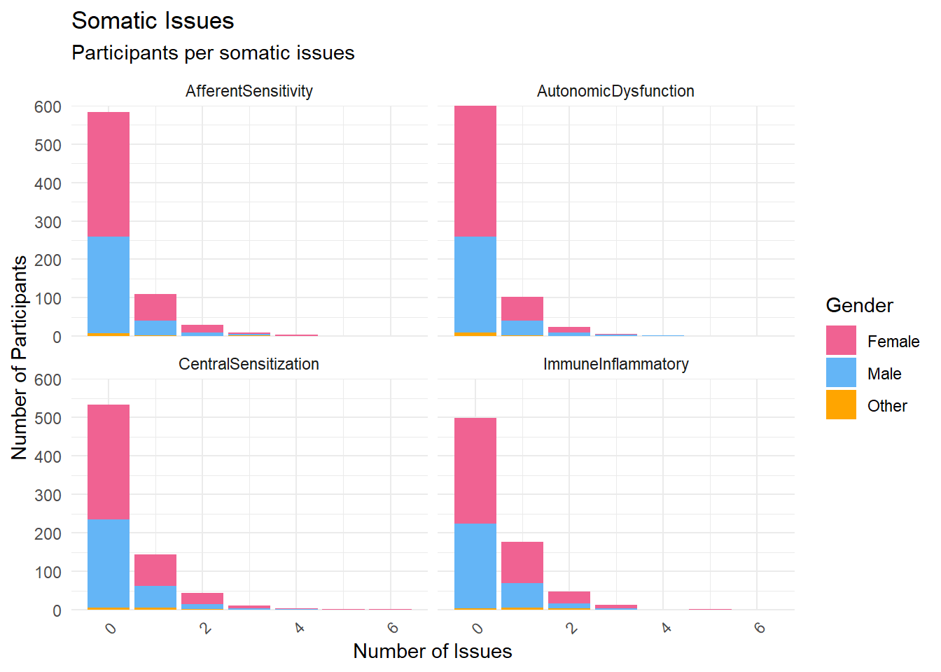

Code

# 
# p2 <- df |> 
#   select(starts_with("Disorders_Somatic_"), Gender, Participant) |> 
#   select(-ends_with("_N"), Gender, Participant) |>
#   pivot_longer(starts_with("Disorders_Somatic_")) |> 
#   summarize(n = n(), .by=c("name", "value", "Gender")) |> 
#   filter(value == TRUE) |> 
#   ggplot(aes(x = name, y=n, fill=Gender)) +
#   geom_bar(stat="identity") +
#   scale_fill_manual(values = c("Male"= "#64B5F6", "Female"= "#F06292", "Other"="orange", "Missing"="brown")) +
#   scale_y_continuous(expand = c(0, 0)) +
#   labs(title = "Somatic Issues", y = "Number of Participants", subtitle = "Participants per somatic issues", x="Type") +
#   theme_minimal() +
#   theme(axis.text.x = element_text(angle = 45, hjust = 1)) 
# p2

Code

p1 <- df |> 
  ggplot(aes(x = Wearables_Number)) +
  geom_bar() +
  scale_x_continuous(breaks = c(0:max(df$Wearables_Number)), expand=c(0, 0)) +
  scale_y_continuous(expand = c(0, 0)) +
  labs(title = "Number of Wearable Devices", y = "Number of Participants", x="Number Owned") +
  theme(axis.text.x = element_text(angle = 45, hjust = 1)) +
  theme_minimal()


p2 <- df |> 
  select(contains("Wearables"), -contains("Importance"), -Wearables_Number) |> 
  pivot_longer(everything()) |> 
  summarize(n = n(), .by=c("name", "value")) |> 
  mutate(value = fct_relevel(value, "Not owning", "Never", "Very rarely", "A few times per week", "Once a day", "A few times per day", "A few times per hour"),
         name = str_remove(name, "Wearables_")) |> 
  ggplot(aes(x=value, y=n, fill=name)) +
  geom_bar(stat = "identity") +
  labs(x = "Usage frequency", y = "") +
  theme_minimal() +
  theme(axis.text.x = element_text(angle = 45, hjust = 1))


get_databubble <- function(df, var="Heart") {
  x <- paste0("Wearables_", var)
  y <- paste0("Wearables_", var, "Importance")
  dat <- df[df[[x]] != "Not owning", ]
  dat <- summarize(dat, n = n(), .by = all_of(c(x, y)))
  lvl <- c("Never", "Very rarely", "A few times per week", "Once a day", "A few times per day", "A few times per hour")
  dat[[x]] <- factor(dat[[x]], levels=lvl[lvl %in% unique(dat[[x]])])
  names(dat) <- c("Usage", "Importance", "n")
  dat$Device <- var
  dat
}

p3 <- rbind(
  get_databubble(df, "Heart"),
  get_databubble(df, "Sleep"),
  get_databubble(df, "Steps"),
  get_databubble(df, "Weight"),
  get_databubble(df, "CalorieIntake"),
  get_databubble(df, "CaloriesBurnt")
) |> 
  filter(!is.na(Importance)) |> 
  ggplot(aes(x=Usage, y=Importance)) +
  geom_jitter(aes(size = n, color = Device), width = 0.2, height = 0.2, alpha = 0.5) +
  geom_smooth(aes(x=as.numeric(Usage), color = Device), method = "lm", se = FALSE, formula = 'y ~ x') +
  labs(x = "Usage frequency") +
  theme_minimal() +
  theme(axis.text.x = element_text(angle = 45, hjust = 1),
        legend.position = "none")

p1 / p2 / p3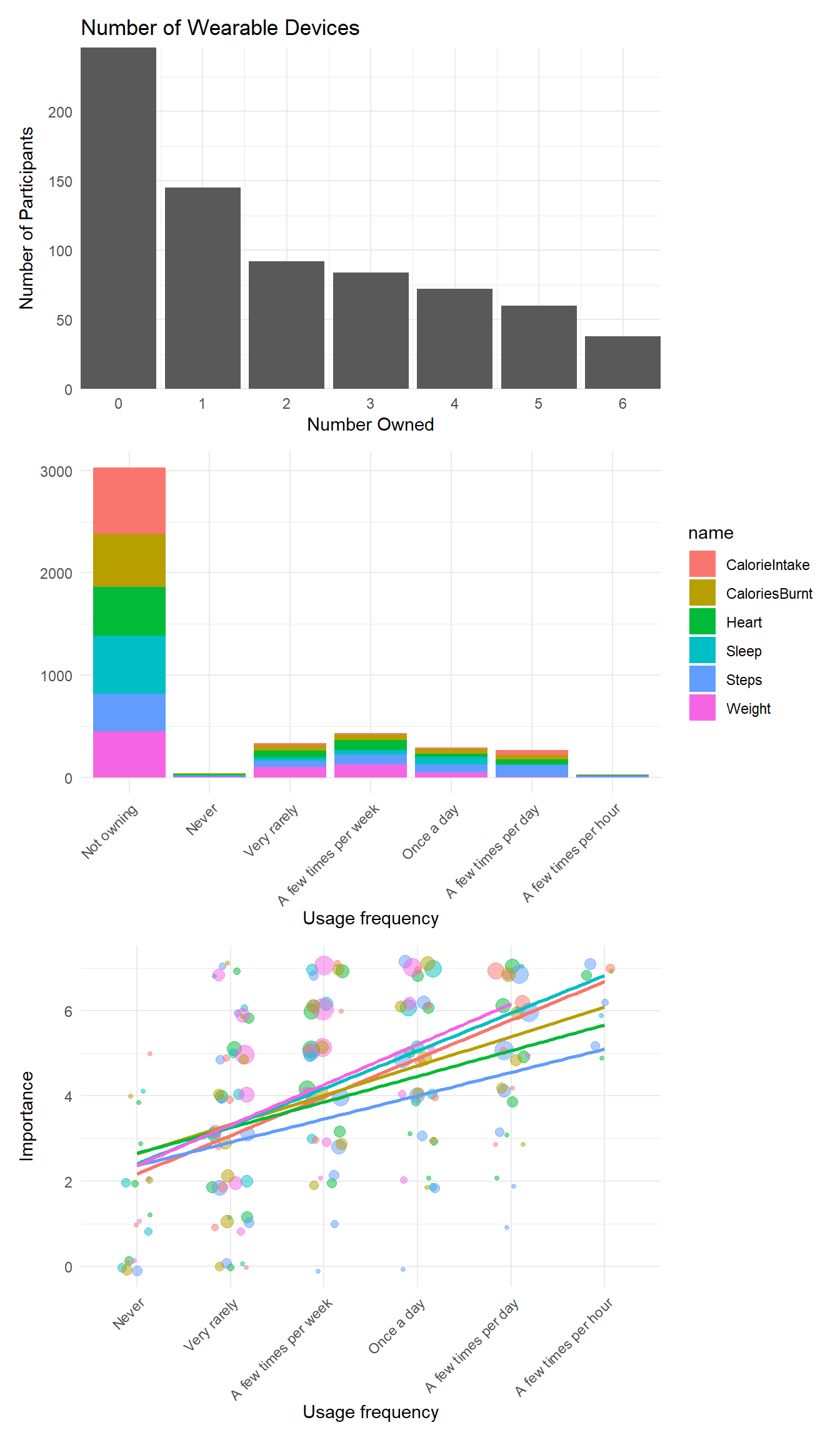

Save

Code

df |> 
  select(-contains("AttentionCheck")) |> 
  write.csv("../data/data_participants.csv", row.names = FALSE)