Code
library(tidyverse)
library(easystats)
library(patchwork)
library(ggside)
library(EGAnet)
library(tidygraph)
library(ggraph)
set.seed(42)
Sys.setenv(CHROMOTE_CHROME = "C:\\Program Files (x86)\\Microsoft\\Edge\\Application\\msedge.exe")library(tidyverse)
library(easystats)
library(patchwork)
library(ggside)
library(EGAnet)
library(tidygraph)
library(ggraph)
set.seed(42)
Sys.setenv(CHROMOTE_CHROME = "C:\\Program Files (x86)\\Microsoft\\Edge\\Application\\msedge.exe")df <- read.csv("../data/data_participants.csv") |>
rename(MINT_Urin_1 = MINT_Deficit_Urin_1,
MINT_Urin_2 = MINT_Deficit_Urin_2,
MINT_Urin_3 = MINT_Deficit_Urin_3,
MINT_CaCo_1 = MINT_Deficit_CaCo_4,
MINT_CaCo_2 = MINT_Deficit_CaCo_5,
MINT_CaCo_3 = MINT_Deficit_CaCo_6,
MINT_CaNo_1 = MINT_Deficit_CaNo_7,
MINT_CaNo_2 = MINT_Deficit_CaNo_8,
MINT_CaNo_3 = MINT_Deficit_CaNo_9,
MINT_Olfa_1 = MINT_Deficit_Olfa_10,
MINT_Olfa_2 = MINT_Deficit_Olfa_11,
MINT_Olfa_3 = MINT_Deficit_Olfa_12,
MINT_Sati_1 = MINT_Deficit_Sati_13,
MINT_Sati_2 = MINT_Deficit_Sati_14,
MINT_Sati_3 = MINT_Deficit_Sati_15,
MINT_SexS_1 = MINT_Awareness_SexS_19,
MINT_SexS_2 = MINT_Awareness_SexS_20,
MINT_SexS_3 = MINT_Awareness_SexS_21,
MINT_SexO_1 = MINT_Awareness_SexO_22,
MINT_SexO_2 = MINT_Awareness_SexO_23,
MINT_SexO_3 = MINT_Awareness_SexO_24,
MINT_UrSe_1 = MINT_Awareness_UrSe_25,
MINT_UrSe_2 = MINT_Awareness_UrSe_26,
MINT_UrSe_3 = MINT_Awareness_UrSe_27,
MINT_RelA_1 = MINT_Awareness_RelA_28,
MINT_RelA_2 = MINT_Awareness_RelA_29,
MINT_RelA_3 = MINT_Awareness_RelA_30,
MINT_StaS_1 = MINT_Awareness_StaS_31,
MINT_StaS_2 = MINT_Awareness_StaS_32,
MINT_StaS_3 = MINT_Awareness_StaS_33,
MINT_ExAc_1 = MINT_Awareness_ExAc_34,
MINT_ExAc_2 = MINT_Awareness_ExAc_35,
MINT_ExAc_3 = MINT_Awareness_ExAc_36,
MINT_Card_1 = MINT_Sensitivity_Card_37,
MINT_Card_2 = MINT_Sensitivity_Card_38,
MINT_Card_3 = MINT_Sensitivity_Card_39,
MINT_Resp_1 = MINT_Sensitivity_Resp_40,
MINT_Resp_2 = MINT_Sensitivity_Resp_41,
MINT_Resp_3 = MINT_Sensitivity_Resp_42,
MINT_Gast_1 = MINT_Sensitivity_Gast_46,
MINT_Gast_2 = MINT_Sensitivity_Gast_47,
MINT_Gast_3 = MINT_Sensitivity_Gast_48,
MINT_Derm_1 = MINT_Sensitivity_Derm_49,
MINT_Derm_2 = MINT_Sensitivity_Derm_50,
MINT_Derm_3 = MINT_Sensitivity_Derm_51)
colors <- c(Mint="#00BCD4", metaMint="#673AB7", miniMint="#26A36C", microMint="#8BC34A",
IAS="#F44336", MAIA="#FFAD04", iMAIA="#FF7811", BPQ="#795548")items <- select(df, starts_with("MINT_"))
names(items) <- str_remove(names(items), "MINT_")See the list of item labels in the code below.
labels <- list(
MINT_Urin_1 = "I sometimes feel like I need to urinate or defecate but when I go to the bathroom I produce less than I expected",
MINT_Urin_2 = "I often feel the need to urinate even when my bladder is not full",
MINT_Urin_3 = "Sometimes I am not sure whether I need to go to the toilet or not (to urinate or defecate)",
MINT_CaCo_1 = "Sometimes my breathing becomes erratic or shallow and I often don't know why",
MINT_CaCo_2 = "I often feel like I can't get enough oxygen by breathing normally",
MINT_CaCo_3 = "Sometimes my heart starts racing and I often don't know why",
MINT_CaNo_1 = "I often only notice how I am breathing when it becomes loud",
MINT_CaNo_2 = "I only notice my heart when it is thumping in my chest",
MINT_CaNo_3 = "I often only notice how I am breathing when my breathing becomes shallow or irregular",
MINT_Olfa_1 = "I often check the smell of my armpits",
MINT_Olfa_2 = "I often check the smell of my own breath",
MINT_Olfa_3 = "I often check the smell of my farts",
MINT_Sati_1 = "I don't always feel the need to eat until I am really hungry",
MINT_Sati_2 = "Sometimes I don't realise I was hungry until I ate something",
MINT_Sati_3 = "I don't always feel the need to drink until I am really thirsty",
# MINT_SexA_16 = "I always feel in my body if I am sexually aroused",
# MINT_SexA_17 = "I can always tell that I am sexually aroused from the way I feel inside",
# MINT_SexA_18 = "I always know when I am sexually aroused",
MINT_SexS_1 = "During sex or masturbation, I often feel very strong sensations coming from my genital areas",
MINT_SexS_2 = "When I am sexually aroused, I often notice specific sensations in my genital area (e.g., tingling, warmth, wetness, stiffness, pulsations)",
MINT_SexS_3 = "My genital organs are very sensitive to pleasant stimulations",
MINT_SexO_1 = "In general, I am very sensitive to changes in my genital organs",
MINT_SexO_2 = "I can notice even very subtle changes in the state of my genital organs",
MINT_SexO_3 = "I am always very aware of the state of my genital organs, even when I am calm",
MINT_UrSe_1 = "In general, I am very aware of the sensations that are happening when I am urinating",
MINT_UrSe_2 = "In general, I am very aware of the sensations that are happening when I am defecating",
MINT_UrSe_3 = "I often experience a pleasant sensation when relieving myself when urinating or defecating)",
MINT_RelA_1 = "I always know when I am relaxed",
MINT_RelA_2 = "I always feel in my body if I am relaxed",
MINT_RelA_3 = "My body is always in the same specific state when I am relaxed",
MINT_StaS_1 = "Being relaxed is a very different bodily feeling compared to other states (e.g., feeling anxious, sexually aroused or after exercise)",
MINT_StaS_2 = "Being sexually aroused is a very different bodily feeling compared to other states (e.g., feeling anxious, relaxed, or after physical exercise)",
MINT_StaS_3 = "Being anxious is a very different bodily feeling compared to other states (e.g., feeling sexually aroused, relaxed or after exercise)",
MINT_ExAc_1 = "I can always accurately feel when I am about to burp",
MINT_ExAc_2 = "I can always accurately feel when I am about to fart",
MINT_ExAc_3 = "I can always accurately feel when I am about to sneeze",
MINT_Card_1 = "In general, I am very sensitive to changes in my heart rate",
MINT_Card_2 = "I can notice even very subtle changes in the way my heart beats",
MINT_Card_3 = "I often notice changes in my heart rate",
MINT_Resp_1 = "I can notice even very subtle changes in my breathing",
MINT_Resp_2 = "I am always very aware of how I am breathing, even when I am calm",
MINT_Resp_3 = "In general, I am very sensitive to changes in my breathing",
# MINT_Sign_43 = "When something important is happening in my life, I can feel immediately feel changes in my heart rate",
# MINT_Sign_44 = "When something important is happening in my life, I can immediately feel changes in my breathing",
# MINT_Sign_45 = "When something important is happening in my life, I can feel it in my body",
MINT_Gast_1 = "I can notice even very subtle changes in what my stomach is doing",
MINT_Gast_2 = "In general, I am very sensitive to what my stomach is doing",
MINT_Gast_3 = "I am always very aware of what my stomach is doing, even when I am calm",
MINT_Derm_1 = "In general, my skin is very sensitive",
MINT_Derm_2 = "My skin is susceptible to itchy fabrics and materials",
MINT_Derm_3 = "I can notice even very subtle stimulations to my skin (e.g., very light touches)"
# MINT_SexC_52 = "When I am sexually aroused, I often feel changes in the way my heart beats (e.g., faster or stronger)",
# MINT_SexC_53 = "When I am sexually aroused, I often feel changes in my breathing (e.g., faster, shallower, or less regular)",
# MINT_SexC_54 = "When I am sexually aroused, I often feel changes in my temperature (e.g., feeling warm or cold)"
)cleanlabels <- function(x, qname=FALSE) {
is_factor <- FALSE
if(is.factor(x)) {
is_factor <- TRUE
vec <- x
x <- levels(x)
}
x <- x |>
str_replace("MINT_", ifelse(qname, "MINT - ", "")) |>
str_replace("MAIA_", ifelse(qname, "MAIA - ", "")) |>
str_replace("_", " - ")
if(is_factor) {
levels(vec) <- x
return(vec)
}
x
}Additionally to EGA, we explored Hierarchical Clustering to see if the results are consistent.
ega1 <- bootEGA(
items,
EGA.type = "hierEGA",
model = "glasso", # BGGM
algorithm = "leiden",
allow.singleton = TRUE,
type="resampling",
plot.itemStability=FALSE,
typicalStructure=TRUE,
plot.typicalGraph=FALSE,
iter=500,
seed=3, ncores = 4)
save(ega1, file="models/ega1.RData")load("models/ega1.RData")
itemstability <- EGAnet::itemStability(ega1, IS.plot=FALSE)
plot(itemstability)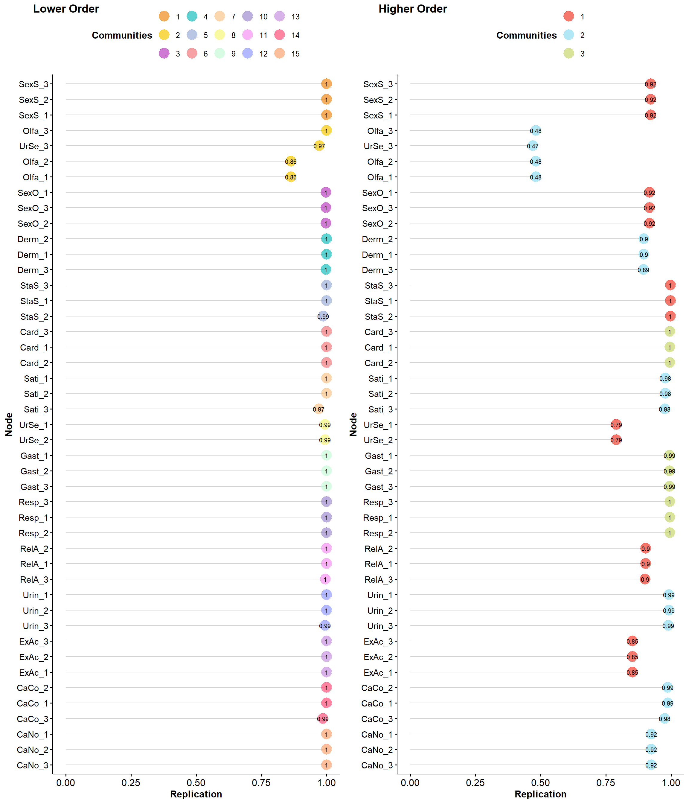
hclust <- pvclust::pvclust(items,
method.hclust = "ward.D2",
method.dist = "correlation",
nboot = 1000, quiet=TRUE, parallel=TRUE)
plot(hclust, hang = -1, cex = 0.5)
pvclust::pvrect(hclust, alpha=0.95, max.only=TRUE)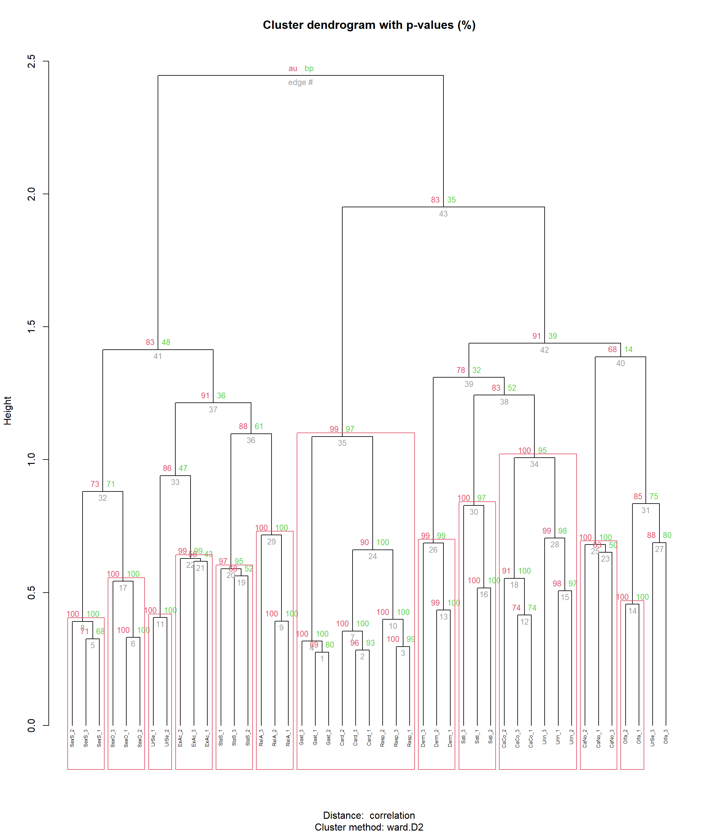
To help us in confirming which clusters to keep or to remove, we empirically tested the “importance” (normalized R2) of each cluster in predicting various outcomes present in our dataset, and aggregating the average importance of each cluster different categories of outcomes. This approach yielded patterns which highlighted some clusters as providing a unique contribution (e.g., Olfa and Sati).
rbind(rez, grandave) |>
select(-Group, -Rank) |>
pivot_wider(names_from = "Outcome", values_from = "R2") |>
mutate(Group = case_when(
Dimension %in% c("Card", "Resp", "Gast", "CardRespGast", "CardResp", "CardGast") ~ "Visceral",
Dimension %in% c("RelA", "SexS", "ExaC", "StaS", "SexO", "UrSe") ~ "sensitivity",
Dimension %in% c("CaCo", "Urin", "Derm", "Olfa", "Sati", "CaNo") ~ "Deficit",
.default = "Other")) |>
select(Group, Dimension, Average, Interoception, Biofeedback, ER,
Primals, Alexithymia, Dissociative, Mood,
Physical, Mental, Lifestyle) |>
arrange(Group, desc(Average)) |>
# select(-Group) |>
gt::gt() |>
gt::data_color(
columns = -c(Dimension, Group),
palette = c("white", "green"),
domain = c(0, 1)
) |>
gt::fmt_number() |>
gt::tab_header(
title = "Variable Importance",
subtitle = "Normalized Predictive Power (R2)"
) |>
gt::tab_row_group(
label = "Sensitivity",
rows = Group == "sensitivity"
) |>
gt::tab_row_group(
label = "Interoception",
rows = Group == "Visceral"
) |>
gt::tab_row_group(
label = "Deficit",
rows = Group == "Deficit"
) |>
gt::cols_hide(Group)| Variable Importance | |||||||||||
|---|---|---|---|---|---|---|---|---|---|---|---|
| Normalized Predictive Power (R2) | |||||||||||
| Dimension | Average | Interoception | Biofeedback | ER | Primals | Alexithymia | Dissociative | Mood | Physical | Mental | Lifestyle |
| Deficit | |||||||||||
| CaCo | 0.62 | 0.10 | 0.05 | 0.32 | 0.77 | 1.00 | 1.00 | 1.00 | 0.64 | 0.72 | 0.76 |
| Urin | 0.43 | 0.09 | 0.20 | 0.07 | 0.54 | 0.64 | 0.52 | 0.61 | 0.74 | 0.45 | 0.22 |
| Derm | 0.32 | 0.06 | 0.01 | 0.15 | 0.35 | 0.29 | 0.20 | 0.34 | 0.87 | 0.59 | 0.08 |
| Olfa | 0.25 | 0.09 | 0.42 | 0.22 | 0.46 | 0.29 | 0.16 | 0.22 | 0.03 | 0.20 | 0.00 |
| Sati | 0.24 | 0.01 | 0.01 | 0.10 | 0.31 | 0.56 | 0.36 | 0.20 | 0.06 | 0.23 | 0.53 |
| CaNo | 0.05 | 0.01 | 0.01 | 0.05 | 0.00 | 0.10 | 0.01 | 0.06 | 0.02 | 0.03 | 0.20 |
| Interoception | |||||||||||
| CardRespGast | 0.32 | 0.78 | 0.81 | 0.26 | 0.11 | 0.04 | 0.08 | 0.19 | 0.28 | 0.22 | 0.01 |
| CardResp | 0.31 | 0.70 | 0.80 | 0.19 | 0.08 | 0.05 | 0.09 | 0.21 | 0.20 | 0.13 | 0.01 |
| CardGast | 0.28 | 0.62 | 0.73 | 0.19 | 0.10 | 0.03 | 0.07 | 0.19 | 0.36 | 0.23 | 0.01 |
| Card | 0.28 | 0.48 | 0.67 | 0.06 | 0.07 | 0.05 | 0.09 | 0.23 | 0.22 | 0.13 | 0.00 |
| Resp | 0.25 | 0.70 | 0.62 | 0.26 | 0.07 | 0.04 | 0.06 | 0.13 | 0.10 | 0.15 | 0.03 |
| Gast | 0.17 | 0.43 | 0.26 | 0.17 | 0.08 | 0.00 | 0.02 | 0.06 | 0.12 | 0.07 | 0.03 |
| Sensitivity | |||||||||||
| RelA | 0.54 | 0.77 | 0.49 | 0.92 | 0.79 | 0.57 | 0.47 | 0.29 | 0.21 | 0.22 | 0.51 |
| SexS | 0.23 | 0.28 | 0.54 | 0.07 | 0.22 | 0.15 | 0.15 | 0.03 | 0.02 | 0.08 | 0.41 |
| UrSe | 0.21 | 0.36 | 0.66 | 0.40 | 0.14 | 0.01 | 0.00 | 0.00 | 0.03 | 0.02 | 0.07 |
| ExaC | 0.20 | 0.16 | 0.12 | 0.11 | 0.33 | 0.10 | 0.09 | 0.03 | 0.04 | 0.17 | 0.08 |
| SexO | 0.18 | 0.43 | 0.48 | 0.23 | 0.03 | 0.00 | 0.00 | 0.01 | 0.00 | 0.02 | 0.19 |
| StaS | 0.16 | 0.21 | 0.13 | 0.04 | 0.10 | 0.16 | 0.28 | 0.02 | 0.02 | 0.08 | 0.18 |
rbind(rez, grandave) |>
select(-Group, -R2) |>
pivot_wider(names_from = "Outcome", values_from = "Rank") |>
mutate(Group = case_when(
Dimension %in% c("Card", "Resp", "Gast", "CardRespGast", "CardResp", "CardGast") ~ "Visceral",
Dimension %in% c("RelA", "SexS", "ExaC", "StaS", "SexO", "UrSe") ~ "sensitivity",
Dimension %in% c("CaCo", "Urin", "Derm", "Olfa", "Sati", "CaNo") ~ "Deficit",
.default = "Other")) |>
datawizard::data_relocate(select=c("Group", "Dimension", "Average", "Interoception")) |>
arrange(Group, Average) |>
gt::gt() |>
# gt::fmt_number(columns = "Average") |>
gt::data_color(
columns = -c(Dimension, Group),
palette = c("green", "white"),
domain = c(1, 18)
) |>
gt::opt_interactive(page_size_default=20)hclust2 <- rez |>
filter(Group != Outcome) |>
select(-Group, -Rank) |>
pivot_wider(names_from = "Dimension", values_from = "R2") |>
select(-Outcome) |>
pvclust::pvclust(
method.hclust = "average",
method.dist = "correlation",
nboot = 1000, quiet=TRUE, parallel=TRUE)
plot(hclust2, hang = -1, cex = 0.5)
pvclust::pvrect(hclust2, alpha=0.95, max.only=TRUE)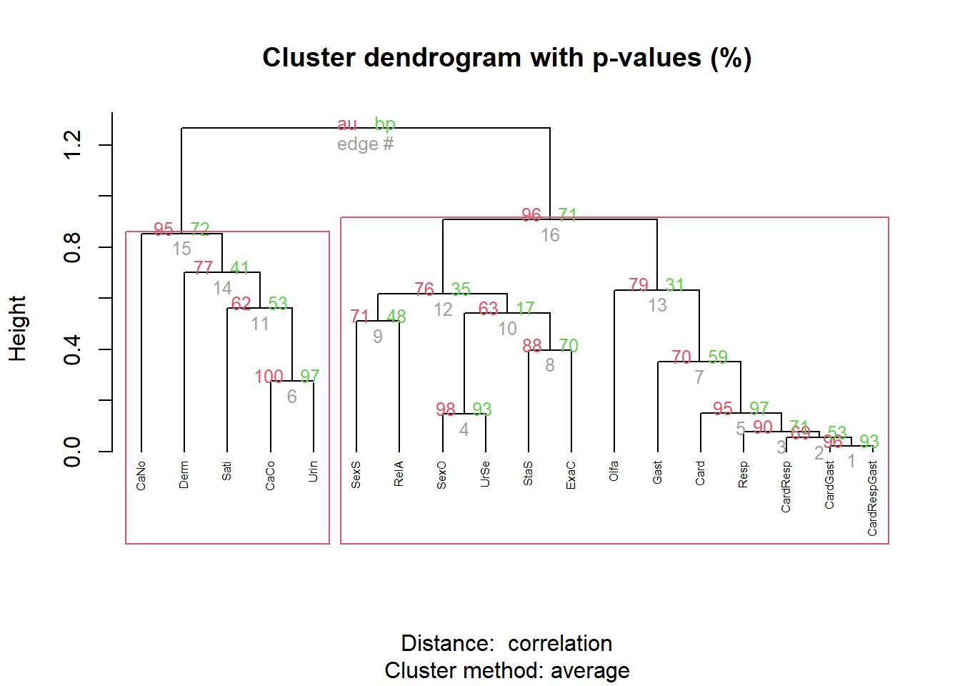
Initially, we fought about also removing Olfa and Sati to provide a more parsimonious and balanced final set, but they seem to withhold interesting value.
items <- items |>
select(
-contains("UrSe"), # Unstable item
-contains("StaS"), # Too vague and overlapping
-contains("SexO"), # Overalapping with SexS
-contains("CaNo") # Overlap with CaCo
# -contains("Olfa"), # Unstable metacluster
# -contains("Sati")
)ega2 <- bootEGA(
items,
EGA.type = "hierEGA",
model = "glasso", # BGGM
algorithm = "leiden",
# consensus.method = "lowest_tefi",
allow.singleton = TRUE,
type="resampling",
plot.itemStability=FALSE,
typicalStructure=TRUE,
plot.typicalGraph=FALSE,
iter=500,
seed=3, ncores = 4)
save(ega2, file="models/ega2.RData")load("models/ega2.RData")
# EGAnet::dimensionStability(ega)
itemstability <- EGAnet::itemStability(ega2, IS.plot=FALSE)
p_stab <- plot(itemstability)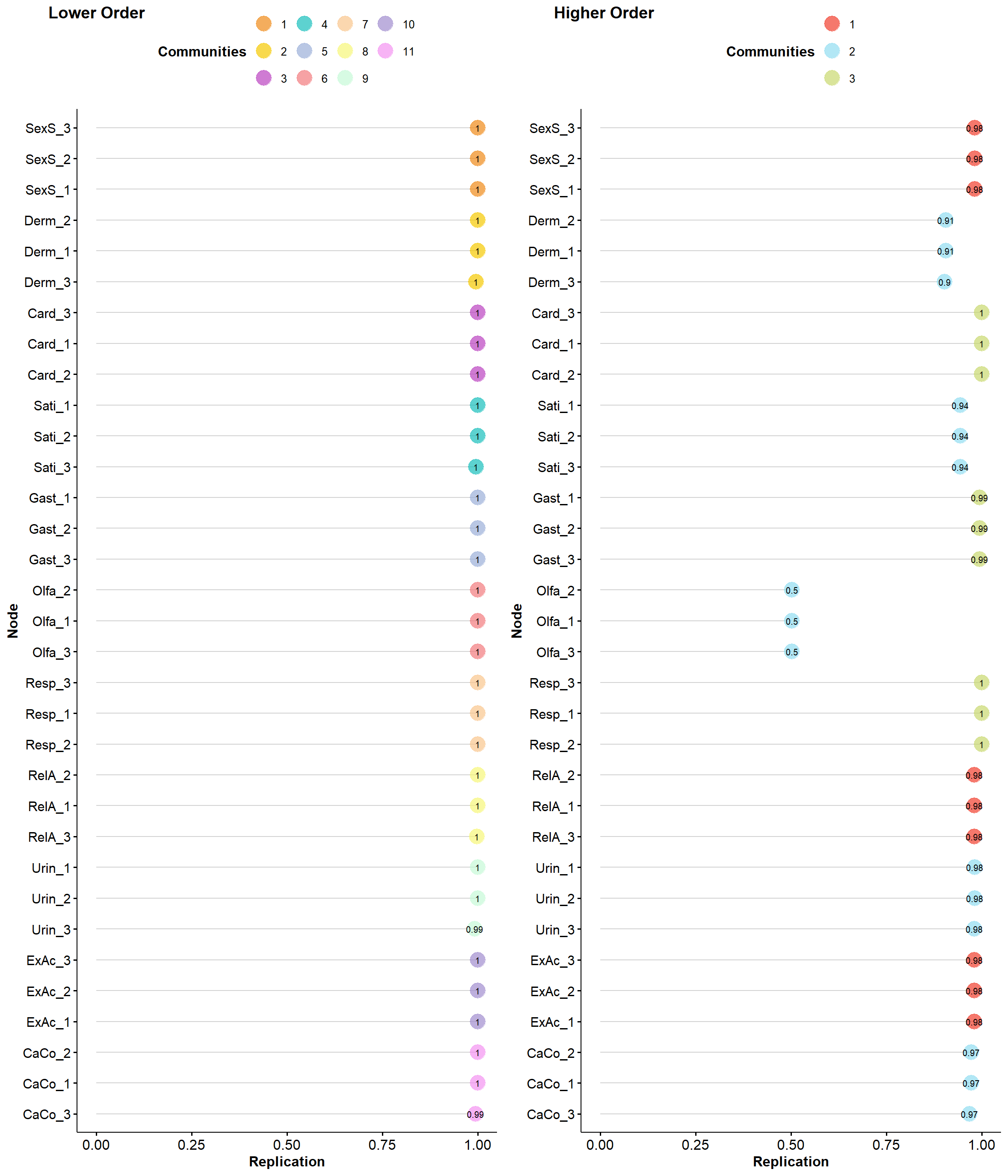
p_stab
ega2$EGA[1;m[4;mLower Order
[0m[0mModel: GLASSO (EBIC with gamma = 0.5)
Correlations: auto
Lambda: 0.07576903751863 (n = 100, ratio = 0.1)
Number of nodes: 33
Number of edges: 183
Edge density: 0.347
Non-zero edge weights:
M SD Min Max
0.072 0.116 -0.116 0.469
----
Consensus Method: Most Common (1000 iterations)
Algorithm: Louvain
Order: Lower
Number of communities: 11
SexS_3 Derm_2 Card_3 SexS_2 Sati_1 Sati_2 Card_1 Derm_3 Gast_1 Olfa_2 Gast_2
1 2 3 1 4 4 3 2 5 6 5
SexS_1 Resp_3 Resp_1 RelA_3 Urin_1 Olfa_1 RelA_2 Olfa_3 RelA_1 ExAc_3 Urin_3
1 7 7 8 9 6 8 6 8 10 9
Derm_1 CaCo_3 CaCo_2 ExAc_2 Card_2 Gast_3 Sati_3 Urin_2 ExAc_1 CaCo_1 Resp_2
2 11 11 10 3 5 4 9 10 11 7
----
Unidimensional Method: Louvain
Unidimensional: No
----
TEFI: -28.818
------------
[1;m[4;mHigher Order
[0m[0mModel: GLASSO (EBIC with gamma = 0.5)
Correlations: auto
Lambda: 0.0686498536738075 (n = 100, ratio = 0.1)
Number of nodes: 11
Number of edges: 40
Edge density: 0.727
Non-zero edge weights:
M SD Min Max
0.075 0.107 -0.176 0.478
----
Algorithm: Leiden with Modularity
Number of communities: 3
01 02 03 04 05 06 07 08 09 10 11
1 2 3 2 3 2 3 1 2 1 2
----
Unidimensional Method: Louvain
Unidimensional: No
----
TEFI: -48.414
----
Generalized TEFI: -77.232
----
Interpretation: Based on lower (-28.818) and higher (-48.414) TEFI, there is better fit for a bifactor structure than correlated lower order factor structuremake_loadingtable <- function(x) {
t <- as.data.frame(x) |>
datawizard::data_addprefix("C")
t$Cluster <- colnames(t)[max.col(t, ties.method='first')]
t |>
rownames_to_column(var="Item") |>
rowwise() |>
mutate(Max = max(c_across(-c(Item, Cluster)))) |>
arrange(Cluster, desc(Max)) |>
as.data.frame()
}
dimensions <- list(
C01 = "SexS", # Sexual Arousal Sensitivity
C02 = "Derm", # Dermal Hypersensitivity
C03 = "Card", # Cardioception
C04 = "Sati", # Satiety Awareness
C05 = "Gast", # Gastroception
C06 = "Olfa", # Olfactory Compensation
C07 = "Resp", # Respiroception
C08 = "RelA", # Relaxation Awareness
C09 = "Urin", # Urointestinal Inaccuracy
C10 = "ExAc", # Expulsion Accuracy
C11 = "CaCo" # Cardiorespiratory Confusion
# C01 = "C01",
# C02 = "C02",
# C03 = "C03",
# C04 = "C04",
# C05 = "C05",
# C06 = "C06",
# C07 = "C07",
# C08 = "C08",
# C09 = "C09",
# C10 = "C10",
# C11 = "C11",
# C12 = "C12"
)
higher <- make_loadingtable(t(net.loads(ega2$EGA$higher_order, loading.method="revised")$std)) |>
arrange(Item)
cluster_order <- names(higher)[!names(higher) %in% c("Item", "Cluster", "Max")]
lower <- make_loadingtable(net.loads(ega2$EGA$lower_order, loading.method="revised")$std) |>
select(names(higher)) |>
mutate(Cluster = fct_relevel(Cluster, cluster_order)) |>
arrange(Cluster, desc(Max))
dimensions <- dimensions[names(dimensions) %in% names(lower)]
higher$Item <- paste0("M", higher$Item)
# higher$Label <- c("Interoceptive Deficit", "Interoceptive Awareness", "Interoceptive Sensitivity")
higher$Label <- c("Interoceptive Awareness", "Interoceptive Deficit", "Visceroception")
higher$ID <- ""
lower <- mutate(lower, Label = labels[paste0("MINT_", Item)], ID=Item, Item = 1:n())
tab1 <- rbind(higher, lower) |>
select(-ID) |>
datawizard::data_relocate("Label", after = "Item") |>
datawizard::data_rename(names(dimensions), dimensions[names(dimensions)]) |>
select(-Cluster, -Max) |>
mutate(`|` = "") |>
gt::gt() |>
gt::tab_row_group(
label = "Items",
rows = 1:(nrow(lower) + nrow(higher))
) |>
gt::tab_row_group(
label = "Metaclusters",
rows = 1:nrow(higher)
) |>
gt::data_color(columns=-Item,
method = "numeric",
palette = c("red", "white", "green"),
domain = c(-1, 1)) |>
gt::tab_style(
style = gt::cell_text(size="small", style="italic"),
locations = gt::cells_body(columns="Label", rows=c(4:36))
) |>
gt::tab_style(
style = list(gt::cell_text(weight="bold"),
gt::cell_fill(color = "#F5F5F5")),
locations = list(
gt::cells_row_groups(groups = "Items"),
gt::cells_row_groups(groups = "Metaclusters")
)
) |>
gt::fmt_number(columns=-Item, decimals=2) |>
gt::tab_header(
title = gt::md("**Item Loadings**"),
subtitle = "Node centrality"
) |>
# Metacluster 1
gt::tab_style(
style = gt::cell_fill(color = "#81C784"),
locations = list(
gt::cells_body(columns="Item", rows=c(1))
)
) |>
gt::tab_style(
style = gt::cell_fill(color = "#81C784"),
locations = list(
gt::cells_column_labels(columns = 3),
gt::cells_body(columns="Item", rows=c(4:6))
)
) |>
gt::tab_style(
style = gt::cell_fill(color = "#AED581"),
locations = list(
gt::cells_column_labels(columns = 4),
gt::cells_body(columns="Item", rows=c(7:9))
)
) |>
gt::tab_style(
style = gt::cell_fill(color = "#DCE775"),
locations = list(
gt::cells_column_labels(columns = 5),
gt::cells_body(columns="Item", rows=c(10:12))
)
) |>
gt::tab_style(
style = gt::cell_fill(color = "#BA68C8"),
locations = list(
gt::cells_body(columns="Item", rows=c(2))
)
) |>
gt::tab_style(
style = gt::cell_fill(color = "#BA68C8"),
locations = list(
gt::cells_column_labels(columns = 6),
gt::cells_body(columns="Item", rows=c(13:15))
)
) |>
gt::tab_style(
style = gt::cell_fill(color = "#9575CD"),
locations = list(
gt::cells_column_labels(columns = 7),
gt::cells_body(columns="Item", rows=c(16:18))
)
) |>
gt::tab_style(
style = gt::cell_fill(color = "#7986CB"),
locations = list(
gt::cells_column_labels(columns = 8),
gt::cells_body(columns="Item", rows=c(19:21))
)
) |>
gt::tab_style(
style = gt::cell_fill(color = "#64B5F6"),
locations = list(
gt::cells_column_labels(columns = 9),
gt::cells_body(columns="Item", rows=c(22:24))
)
) |>
gt::tab_style(
style = gt::cell_fill(color = "#4DD0E1"),
locations = list(
gt::cells_column_labels(columns = 10),
gt::cells_body(columns="Item", rows=c(25:27))
)
) |>
gt::tab_style(
style = gt::cell_fill(color = "#FF7811"),
locations = list(
gt::cells_body(columns="Item", rows=c(3))
)
) |>
gt::tab_style(
style = gt::cell_fill(color = "#FFB74D"),
locations = list(
gt::cells_column_labels(columns = 11),
gt::cells_body(columns="Item", rows=c(28:30))
)
) |>
gt::tab_style(
style = gt::cell_fill(color = "#E57373"),
locations = list(
gt::cells_column_labels(columns = 12),
gt::cells_body(columns="Item", rows=c(31:33))
)
) |>
gt::tab_style(
style = gt::cell_fill(color = "#A1887F"),
locations = list(
gt::cells_column_labels(columns = 13),
gt::cells_body(columns="Item", rows=c(34:36))
)
)
tab1| Item Loadings | |||||||||||||
|---|---|---|---|---|---|---|---|---|---|---|---|---|---|
| Node centrality | |||||||||||||
| Item | Label | ExAc | RelA | SexS | CaCo | Urin | Derm | Sati | Olfa | Resp | Card | Gast | | |
| Metaclusters | |||||||||||||
| M1 | Interoceptive Awareness | 0.42 | 0.41 | 0.30 | −0.20 | −0.06 | 0.06 | −0.07 | 0.08 | 0.13 | 0.02 | 0.12 | |
| M2 | Interoceptive Deficit | 0.00 | −0.17 | 0.01 | 0.49 | 0.44 | 0.24 | 0.23 | 0.18 | 0.21 | 0.20 | 0.12 | |
| M3 | Visceroception | 0.02 | 0.15 | 0.02 | 0.20 | 0.01 | 0.11 | 0.00 | 0.13 | 0.60 | 0.58 | 0.33 | |
| Items | |||||||||||||
| 1 | I can always accurately feel when I am about to fart | 0.48 | 0.02 | 0.05 | 0.00 | 0.00 | 0.04 | −0.01 | 0.10 | 0.00 | 0.00 | 0.00 | |
| 2 | I can always accurately feel when I am about to sneeze | 0.48 | 0.09 | 0.01 | 0.00 | 0.00 | 0.04 | 0.00 | 0.00 | 0.00 | 0.00 | 0.00 | |
| 3 | I can always accurately feel when I am about to burp | 0.46 | 0.06 | 0.01 | −0.02 | −0.04 | 0.05 | −0.06 | 0.00 | 0.03 | 0.00 | 0.00 | |
| 4 | I always feel in my body if I am relaxed | 0.02 | 0.59 | 0.02 | −0.04 | 0.00 | 0.00 | −0.01 | 0.00 | 0.04 | 0.00 | 0.03 | |
| 5 | I always know when I am relaxed | 0.10 | 0.58 | 0.03 | −0.10 | −0.07 | 0.00 | −0.03 | −0.01 | 0.03 | 0.03 | 0.02 | |
| 6 | My body is always in the same specific state when I am relaxed | 0.04 | 0.28 | 0.00 | −0.01 | 0.00 | 0.00 | 0.00 | 0.00 | 0.00 | 0.03 | 0.00 | |
| 7 | During sex or masturbation, I often feel very strong sensations coming from my genital areas | 0.01 | 0.03 | 0.65 | −0.05 | −0.04 | 0.00 | 0.00 | 0.00 | 0.00 | 0.00 | 0.00 | |
| 8 | My genital organs are very sensitive to pleasant stimulations | 0.00 | 0.02 | 0.53 | 0.00 | 0.00 | 0.02 | 0.00 | 0.01 | 0.00 | 0.00 | 0.00 | |
| 9 | When I am sexually aroused, I often notice specific sensations in my genital area (e.g., tingling, warmth, wetness, stiffness, pulsations) | 0.08 | 0.02 | 0.53 | 0.00 | 0.01 | 0.03 | 0.00 | 0.02 | 0.00 | 0.01 | 0.02 | |
| 10 | Sometimes my breathing becomes erratic or shallow and I often don't know why | −0.02 | −0.01 | 0.00 | 0.68 | 0.11 | 0.00 | 0.09 | 0.02 | 0.07 | 0.00 | 0.00 | |
| 11 | I often feel like I can't get enough oxygen by breathing normally | 0.00 | −0.07 | −0.04 | 0.39 | 0.04 | 0.04 | 0.02 | 0.02 | 0.06 | 0.04 | 0.00 | |
| 12 | Sometimes my heart starts racing and I often don't know why | 0.00 | −0.07 | 0.00 | 0.37 | 0.06 | 0.05 | 0.03 | 0.00 | 0.00 | 0.16 | 0.00 | |
| 13 | I sometimes feel like I need to urinate or defecate but when I go to the bathroom I produce less than I expected | 0.00 | 0.00 | 0.01 | 0.08 | 0.63 | 0.03 | 0.01 | 0.07 | 0.00 | 0.00 | 0.00 | |
| 14 | I often feel the need to urinate even when my bladder is not full | 0.00 | −0.01 | 0.00 | 0.04 | 0.44 | 0.09 | 0.00 | 0.02 | 0.00 | 0.00 | 0.01 | |
| 15 | Sometimes I am not sure whether I need to go to the toilet or not (to urinate or defecate) | −0.04 | −0.06 | −0.03 | 0.09 | 0.32 | 0.00 | 0.12 | 0.00 | 0.00 | 0.00 | 0.00 | |
| 16 | In general, my skin is very sensitive | 0.00 | 0.00 | 0.00 | 0.01 | 0.00 | 0.70 | 0.02 | 0.00 | 0.04 | 0.00 | 0.01 | |
| 17 | My skin is susceptible to itchy fabrics and materials | 0.00 | 0.00 | 0.00 | 0.07 | 0.07 | 0.46 | 0.01 | 0.01 | 0.00 | 0.00 | 0.01 | |
| 18 | I can notice even very subtle stimulations to my skin (e.g., very light touches) | 0.13 | 0.00 | 0.04 | 0.00 | 0.05 | 0.30 | 0.00 | 0.00 | 0.02 | 0.03 | 0.04 | |
| 19 | I don't always feel the need to eat until I am really hungry | −0.01 | 0.00 | 0.00 | 0.00 | 0.00 | 0.01 | 0.60 | 0.00 | 0.00 | 0.00 | 0.00 | |
| 20 | Sometimes I don't realise I was hungry until I ate something | −0.05 | −0.02 | 0.00 | 0.09 | 0.10 | 0.01 | 0.49 | 0.02 | 0.01 | 0.00 | 0.00 | |
| 21 | I don't always feel the need to drink until I am really thirsty | 0.00 | −0.03 | 0.00 | 0.04 | 0.03 | 0.00 | 0.23 | 0.03 | 0.00 | −0.01 | 0.00 | |
| 22 | I often check the smell of my armpits | 0.00 | −0.01 | 0.00 | 0.02 | 0.03 | 0.00 | 0.04 | 0.59 | 0.04 | 0.03 | 0.00 | |
| 23 | I often check the smell of my own breath | 0.00 | 0.00 | 0.01 | 0.02 | 0.00 | 0.00 | 0.02 | 0.55 | 0.04 | 0.00 | 0.04 | |
| 24 | I often check the smell of my farts | 0.10 | 0.00 | 0.01 | 0.00 | 0.06 | 0.01 | 0.00 | 0.28 | 0.00 | 0.00 | 0.01 | |
| 25 | In general, I am very sensitive to changes in my breathing | 0.00 | 0.04 | 0.00 | 0.06 | 0.00 | 0.07 | 0.00 | 0.02 | 0.54 | 0.15 | 0.02 | |
| 26 | I can notice even very subtle changes in my breathing | 0.03 | 0.03 | 0.00 | 0.03 | 0.00 | 0.00 | 0.00 | 0.01 | 0.54 | 0.14 | 0.02 | |
| 27 | I am always very aware of how I am breathing, even when I am calm | 0.00 | 0.02 | 0.00 | 0.04 | 0.00 | 0.00 | 0.01 | 0.04 | 0.43 | 0.05 | 0.06 | |
| 28 | In general, I am very sensitive to changes in my heart rate | 0.00 | 0.00 | 0.00 | 0.07 | 0.00 | 0.03 | −0.01 | 0.00 | 0.11 | 0.55 | 0.03 | |
| 29 | I often notice changes in my heart rate | 0.00 | 0.00 | 0.01 | 0.14 | 0.00 | 0.00 | 0.00 | 0.03 | 0.08 | 0.53 | 0.01 | |
| 30 | I can notice even very subtle changes in the way my heart beats | 0.00 | 0.07 | 0.00 | 0.01 | 0.00 | 0.00 | 0.00 | 0.00 | 0.17 | 0.45 | 0.05 | |
| 31 | I can notice even very subtle changes in what my stomach is doing | 0.00 | 0.02 | 0.00 | 0.00 | 0.01 | 0.04 | 0.00 | 0.03 | 0.05 | 0.04 | 0.59 | |
| 32 | In general, I am very sensitive to what my stomach is doing | 0.00 | 0.00 | 0.01 | 0.00 | 0.00 | 0.02 | 0.00 | 0.02 | 0.00 | 0.02 | 0.58 | |
| 33 | I am always very aware of what my stomach is doing, even when I am calm | 0.00 | 0.04 | 0.01 | 0.00 | 0.00 | 0.00 | 0.00 | 0.00 | 0.07 | 0.04 | 0.53 | |
gt::gtsave(tab1, "figures/table1.png", vwidth=1660, expand=0, quiet=TRUE)rez <- pvclust::pvclust(items,
method.hclust = "ward.D2",
method.dist = "correlation",
nboot = 1000, quiet=TRUE, parallel=TRUE)
plot(rez, hang = -1, cex = 0.5)
pvclust::pvrect(rez, alpha=0.95, max.only=FALSE)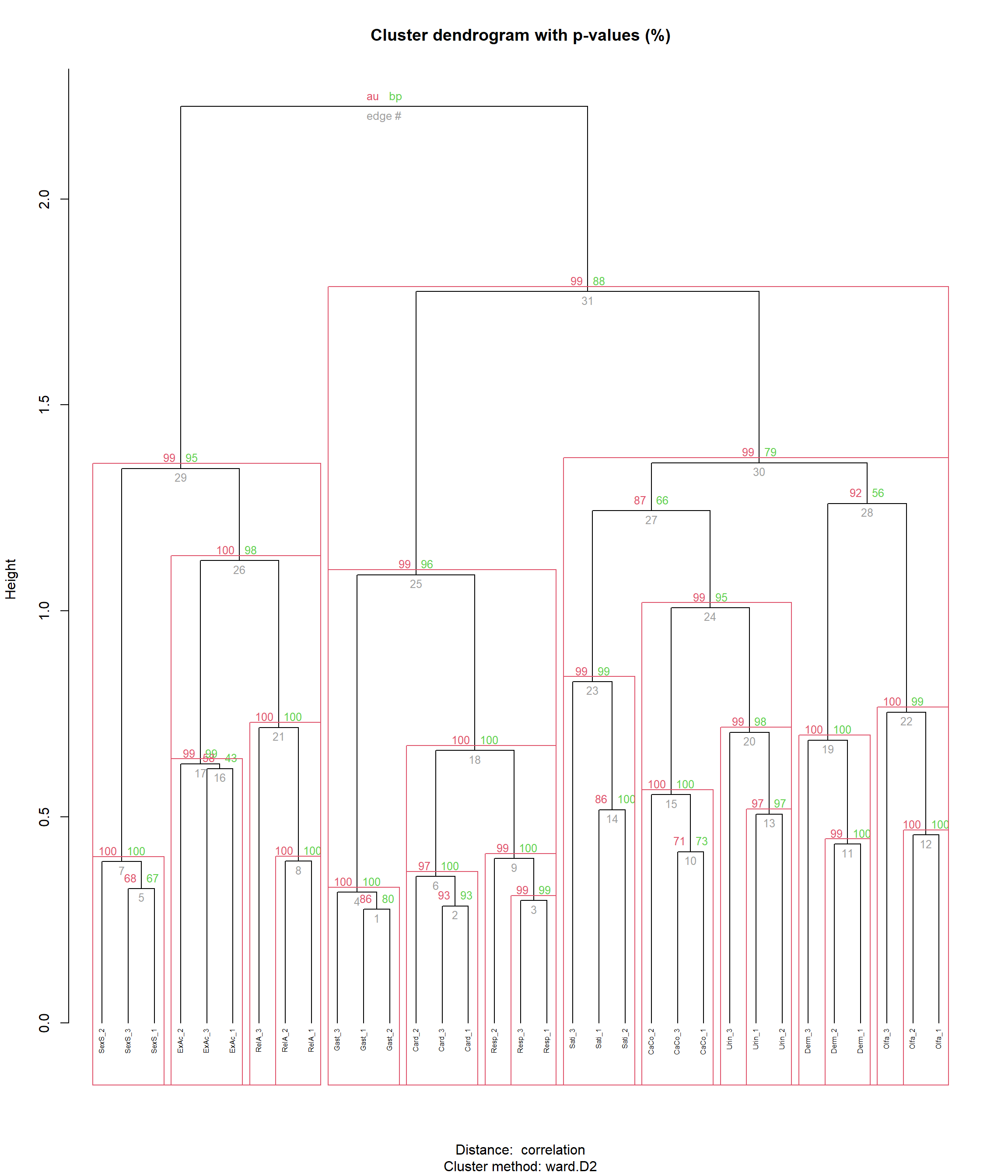
dendrogram <- as.dist(1 - cor(items, use = "pairwise.complete.obs")) |>
hclust(method = "ward.D2") |>
tidygraph::as_tbl_graph()
# Process Nodes
nodes <- as.list(dendrogram)$nodes |>
mutate(Group = case_when(str_detect(label, "Card") ~ "Card",
str_detect(label, "Resp") ~ "Resp",
str_detect(label, "Gast") ~ "Gast",
str_detect(label, "SexS") ~ "SexS",
str_detect(label, "RelA") ~ "RelA",
str_detect(label, "ExAc") ~ "ExAc",
str_detect(label, "Urin") ~ "Urin",
str_detect(label, "CaCo") ~ "CaCo",
str_detect(label, "Derm") ~ "Derm",
str_detect(label, "Olfa") ~ "Olfa",
str_detect(label, "Sati") ~ "Sati",
label == "" ~ "NA",
.default = "Other"),
Size = setNames(lower$Max, lower$ID)[label],
item = label)
nodes$idx <- 1:nrow(nodes)
# Rename accoring to table
items_newnames <- lower |>
separate(ID, into = c("Group", "Item"), sep = "_", remove = FALSE) |>
mutate(Name = paste0(Group, "-", 1:nrow(lower)))
items_newnames <- setNames(items_newnames$Name, items_newnames$ID)
nodes$label <- items_newnames[nodes$label]
nodes$label <- ifelse(is.na(nodes$label), "", nodes$label)
# Central node
max_size <- max(nodes$Size, na.rm = TRUE)
nodes[nodes$height == max(nodes$height), c("Group", "Size")] <- data.frame(Group="Central", Size=2 * max_size)
# Metaclusters
nodes[17, c("Group", "Size")] <- data.frame(Group="Awareness", Size=1.5 * max_size)
nodes[34, c("Group", "Size")] <- data.frame(Group="Visceroception", Size=1.5 * max_size)
nodes[63, c("Group", "Size")] <- data.frame(Group="Deficit", Size=1.5 * max_size)
# Process Edges
edges <- as.list(dendrogram)$edges
edges$linewidth = datawizard::rescale(nodes[edges$from, ]$height, to = c(0.1, 1))
p_hclust <- tbl_graph(nodes = nodes, edges = edges) |>
ggraph(layout = "dendrogram", circular = TRUE) +
# geom_edge_diagonal(strength = 0.7, linewidth = 1) +
geom_edge_elbow2(aes(edge_width=linewidth), color="darkgrey") +
geom_node_point(aes(filter=Group %in% c("Central"), size = Size), color="darkgrey") +
geom_node_point(aes(filter=Group %in% c("Visceroception", "Awareness", "Deficit"), color=Group, size = Size)) +
geom_node_text(aes(
label = ifelse(label != "NA", label, NA),
x = x * 1.07,
y = y * 1.07,
filter = label != "",
angle = ifelse(
x >= 0,
asin(y) * 360 / 2 / pi,
360 - asin(y) * 360 / 2 / pi
),
hjust = ifelse(
x >= 0, 0, 1
))) +
geom_node_point(aes(filter = label != "", color=Group, size=Size), alpha = 1) +
# geom_node_text(aes(label=idx)) + # Debug
scale_edge_width_continuous(range=c(1, 3), guide = "none") +
scale_size_continuous(range=c(3, 11), guide = "none") +
scale_color_manual(values = c(
"Visceroception" = "#FF7811", "Card" = "#F44336", "Resp"="#FF9800", "Gast"="#795548",
"Awareness" = "#4CAF50", "ExAc"="#4CAF50", "RelA"="#8BC34A", "SexS" = "#CDDC39",
"Deficit" = "#9C27B0", "CaCo"="#9C27B0", "Urin" = "#673AB7", "Derm"="#3F51B5",
"Sati" = "#2196F3", "Olfa" = "#00BCD4"),
breaks = c(
"Awareness", "ExAc", "RelA", "SexS",
"Deficit", "CaCo", "Urin", "Derm", "Sati", "Olfa",
"Visceroception", "Resp", "Card", "Gast"
),
labels=c(
"***Awareness***", "ExAc", "RelA", "SexS",
"***Deficit***", "CaCo", "Urin", "Derm", "Sati", "Olfa",
"***Visceroception***", "Resp", "Card", "Gast"
)) +
ggtitle("Hierarchical Clustering", subtitle = "Method = Correlation") +
coord_equal(clip = "off", xlim = c(-1.25, 1.25), ylim = c(-1.25, 1.25)) +
theme_void() +
guides(color = guide_legend(override.aes = list(size = c(7.5, 5, 5, 3.5, 7.5, 5, 5, 3.5, 3.5, 3.5, 7.5, 5, 5, 3.5)))) +
theme(legend.text = ggtext::element_markdown(),
legend.title = element_blank(),
plot.title = element_blank(), #element_text(face="bold")
plot.subtitle = element_blank())
p_hclust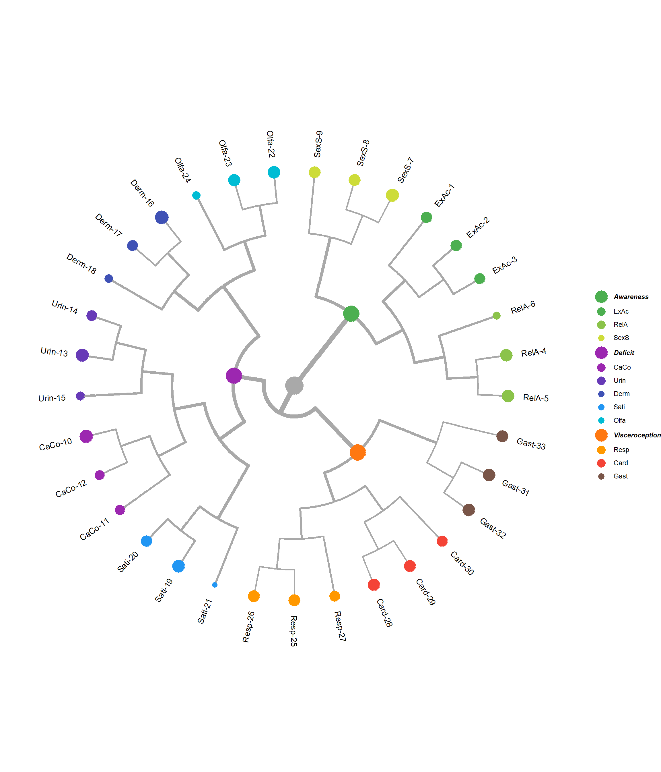
ggsave("figures/fig1a.png", p_stab, width=10, height=10*0.8, dpi=300)
ggsave("figures/fig1b.png", p_hclust, width=8, height=8*0.8, dpi=300)n <- parameters::n_factors(items)
plot(n)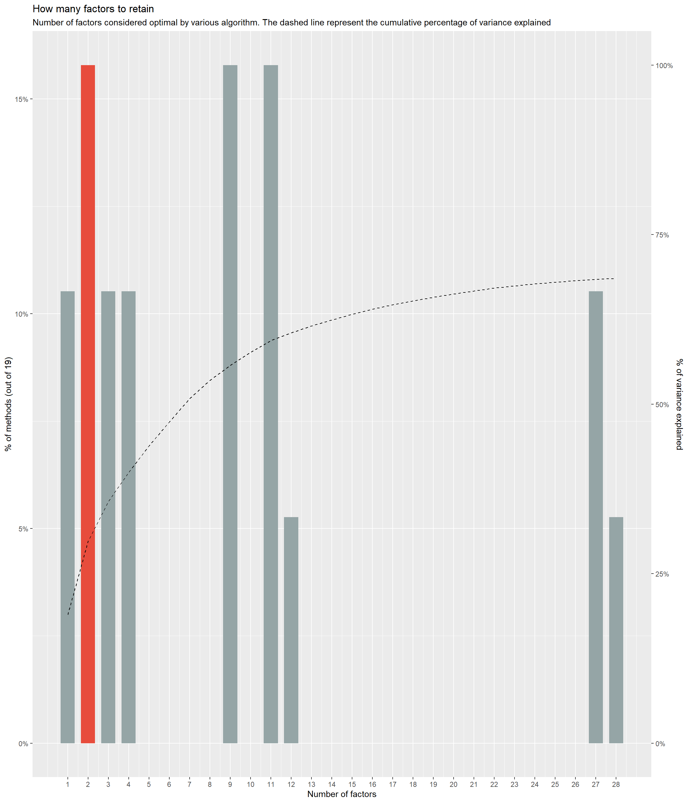
fa <- parameters::factor_analysis(items, n = 9, rotation = "varimax", sort = TRUE)
plot(fa)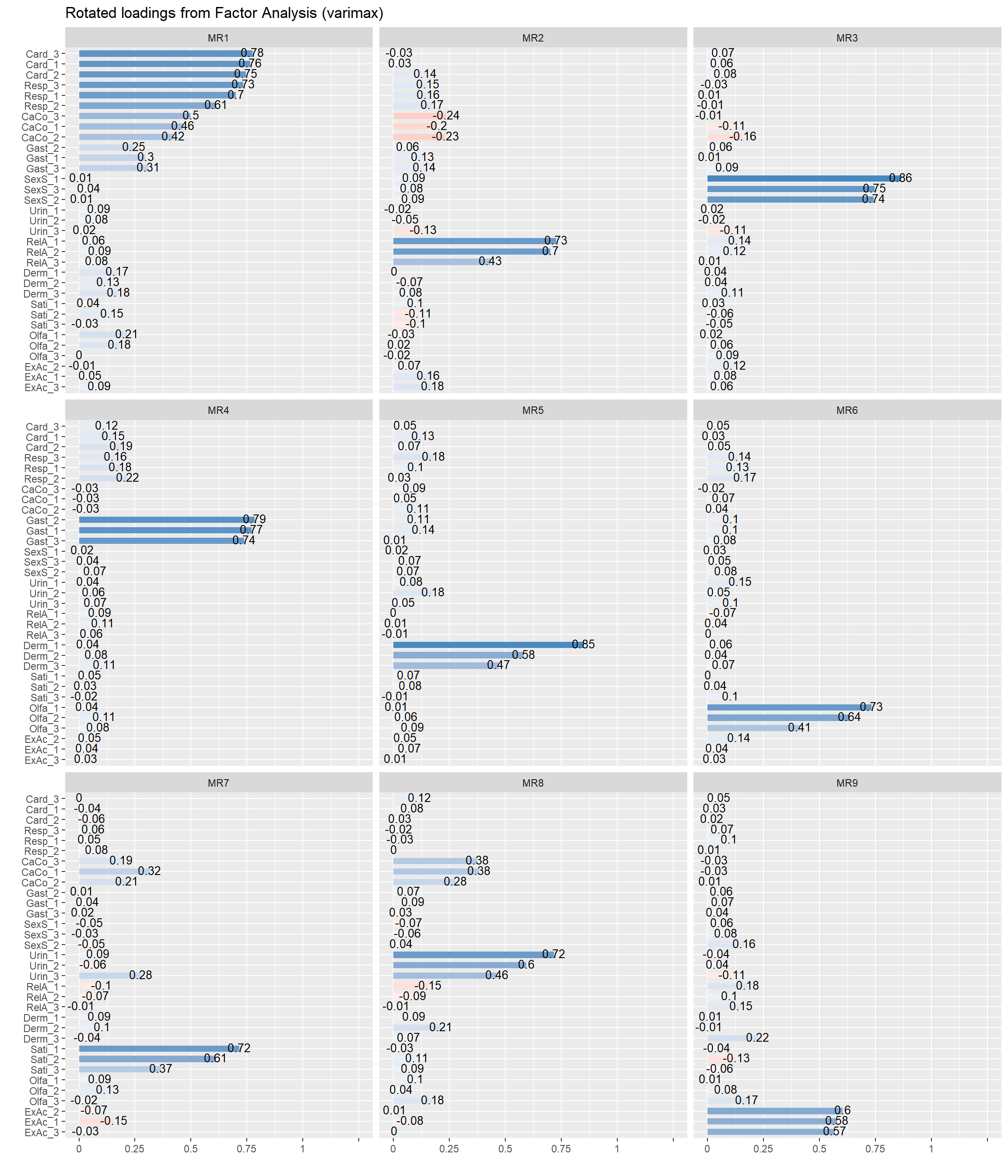
# fa |>
# select(Variable, Uniqueness) |>
# mutate(Group = str_extract(Variable, "^[A-Z][a-z]+")) |>
# mutate(Average = mean(Uniqueness), .by = "Group") |>
# arrange(desc(Average), desc(Uniqueness)) |>
# select(-Average, -Group) |>
# gt::gt() |>
# gt::data_color(
# columns = "Uniqueness",
# palette = c("red", "white", "green"),
# domain = c(0, 1)
# ) # Awareness
df$MINT_SexS <- rowMeans(select(df, starts_with("MINT_SexS_")), na.rm = TRUE)
df$MINT_ExaC <- rowMeans(select(df, starts_with("MINT_ExaC_")), na.rm = TRUE)
df$MINT_RelA <- rowMeans(select(df, starts_with("MINT_RelA_")), na.rm = TRUE)
# df$MINT_StaS <- rowMeans(select(df, starts_with("MINT_StaS_")), na.rm = TRUE)
# df$MINT_SexO <- rowMeans(select(df, starts_with("MINT_SexO_")), na.rm = TRUE)
# df$MINT_UrSe <- rowMeans(select(df, starts_with("MINT_UrSe_")), na.rm = TRUE)
# Deficit
df$MINT_Urin <- rowMeans(select(df, starts_with("MINT_Urin_")), na.rm = TRUE)
df$MINT_CaCo <- rowMeans(select(df, starts_with("MINT_CaCo_")), na.rm = TRUE)
df$MINT_Derm <- rowMeans(select(df, starts_with("MINT_Derm_")), na.rm = TRUE)
# df$MINT_CaNo <- rowMeans(select(df, starts_with("MINT_CaNo_")), na.rm = TRUE)
df$MINT_Sati <- rowMeans(select(df, starts_with("MINT_Sati_")), na.rm = TRUE)
df$MINT_Olfa <- rowMeans(select(df, starts_with("MINT_Olfa_")), na.rm = TRUE)
# Visceral
df$MINT_Resp <- rowMeans(select(df, starts_with("MINT_Resp_")), na.rm = TRUE)
df$MINT_Card <- rowMeans(select(df, starts_with("MINT_Card_")), na.rm = TRUE)
df$MINT_Gast <- rowMeans(select(df, starts_with("MINT_Gast_")), na.rm = TRUE)
df <- df[names(df)[!grepl("MINT_.*[0-9]$", names(df))]]mint <- select(df, starts_with("MINT_"))
metamint <- data.frame(
MINT_Awareness = rowMeans(select(df, MINT_SexS, MINT_ExaC, MINT_RelA)),
MINT_Deficit = rowMeans(select(df, MINT_CaCo, MINT_Urin, MINT_Derm, MINT_Sati, MINT_Olfa)),
MINT_Visceroception = rowMeans(select(df, MINT_Card, MINT_Resp, MINT_Gast))
)
minimint <- data.frame(
MINT_Awareness = rowMeans(select(df, MINT_ExaC, MINT_RelA)),
MINT_Deficit = rowMeans(select(df, MINT_CaCo, MINT_Urin)),
MINT_Visceroception = rowMeans(select(df, MINT_Resp, MINT_Card))
)
micromint <- data.frame(
MINT_ExaC = df$MINT_ExaC,
MINT_CaCo = df$MINT_CaCo,
MINT_Resp = df$MINT_Resp
)make_cor <- function(df1, df2=NULL, qname_x=TRUE, qname_y=TRUE, textsize = 3, xcol = "#424242", ycol="#424242") {
r <- df1 |>
correlation::correlation(data2=df2, p_adjust="none", redundant=ifelse(is.null(df2), TRUE, FALSE)) |>
correlation::cor_sort() |>
mutate(label = ifelse(p < .001, paste0(insight::format_value(r, lead_zero = FALSE, zap_small = TRUE)), ""),
Parameter1 = cleanlabels(Parameter1, qname=qname_x),
Parameter2 = cleanlabels(Parameter2, qname=qname_y))
r[as.character(r$Parameter1) == as.character(r$Parameter2), "label"] <- ""
xnames <- levels(r$Parameter1)
ynames <- levels(r$Parameter2)
xcol <- case_when(
str_detect(xnames, "MINT") ~ "#00838F",
str_detect(xnames, "MAIA") ~ "#EF6C00",
str_detect(xnames, "IAS") ~ "#C62828",
str_detect(xnames, "BPQ") ~ "#795548",
.default = xcol
)
ycol <- case_when(
str_detect(ynames, "MINT") ~ "#00838F",
str_detect(ynames, "MAIA") ~ "#EF6C00",
str_detect(ynames, "IAS") ~ "#C62828",
str_detect(ynames, "BPQ") ~ "#795548",
.default = ycol
)
xbold <- case_when(
xnames %in% c("Awareness", "MINT - Awareness") ~ "bold",
str_detect(xnames, "Visceroception") ~ "bold",
str_detect(xnames, "Deficit") ~ "bold",
.default = "plain"
)
ybold <- case_when(
ynames %in% c("Awareness", "MINT - Awareness") ~ "bold",
str_detect(ynames, "Visceroception") ~ "bold",
str_detect(ynames, "Deficit") ~ "bold",
.default = "plain"
)
r |>
ggplot(aes(x=Parameter1, y=Parameter2, fill=r)) +
geom_tile() +
geom_text(aes(label=label), size=textsize) +
scale_fill_gradient2(low="blue", high="red", mid="white", midpoint=0) +
theme_minimal() +
theme(axis.text.x = element_text(angle = 45, hjust=1, color = xcol, face = xbold),
axis.text.y = element_text(color = ycol, face = ybold),
legend.position = "none",
axis.title = element_blank())
}
p_cormint <- make_cor(cbind(mint, metamint), qname_x = FALSE, qname_y = FALSE, textsize = 2.8,
xcol = "#00838F", ycol = "#00838F") +
labs(title="Correlations between MINT dimensions") +
theme(axis.title = element_blank())
p_cormint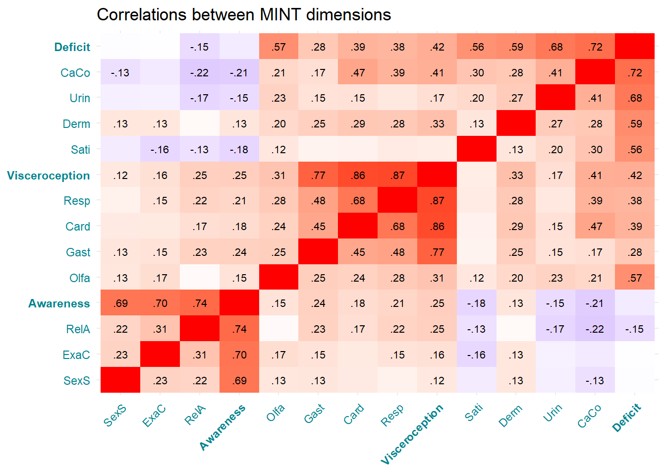
p_corintero <- make_cor(select(df, starts_with("MAIA"), IAS, BPQ),
cbind(mint, metamint), qname_y = FALSE, textsize = 2.8,
ycol = "#00838F") +
labs(title="MINT vs. Other Interoception Questionnaires") +
theme(axis.title = element_blank())
p_corintero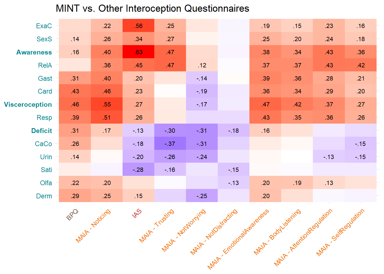
Most correlated dimensions: - IAS: ExAc - Trusting: RelA - Noticing: Resp - Emotional Awareness: Resp - Body Listening: Gast - SelfRegulation: RelA - AttentionRegulation: RelA - BPQ: Card
table_models <- function(models) {
test <- test_performance(models)
table <- compare_performance(models, metrics=c("R2", "BIC"))
test$Model <- NULL
test$Omega2 <- NULL
test$p_Omega2 <- NULL
test$LR <- NULL
test$p_LR <- NULL
test$R2 <- table$R2
test$BIC <- table$BIC
preds <- c()
coefs <- c()
for(m in models){
x <- names(sort(abs(coef(m)[-1]), decreasing=TRUE))
preds <- c(preds, paste0(cleanlabels(x), collapse = ", "))
if(length(coef(m)) == 2) {
coefs <- c(coefs, coef(m)[2])
}
}
test <- datawizard::data_select(test, c("Name", "R2", "BIC", "BF"))
if(length(coefs) == length(models)) test$Coefficient <- coefs
test
}
display_models <- function(table, title = "", subtitle = "") {
numcols <- c("R2", "BIC", "Coefficient")[c("R2", "BIC", "Coefficient") %in% names(table)]
table |>
mutate(BF = format_bf(BF, name = NULL, stars = TRUE)) |>
gt::gt() |>
gt::fmt_number(columns = numcols, decimals = 3) |>
gt::tab_header(title = title, subtitle = subtitle) |>
gt::data_color(
columns = c("R2"),
palette = c("white", "green")
) |>
gt::data_color(
columns = c("BIC"),
palette = c("green", "white")
) |>
gt::opt_interactive(use_compact_mode=TRUE)
}
# Individual predictors ------------------------------------------------------
compare_predictors <- function(outcome="TAS_DIF", family = "linear") {
preds <- c("BPQ", "IAS",
names(select(df, starts_with("MINT"), -matches("[[:digit:]]"))),
names(select(df, starts_with("MAIA"))),
names(metamint))
models <- list()
for(p in preds) {
if(length(unique(df[[outcome]])) > 2) {
if (family == "linear") {
models[[p]] <- lm(as.formula(paste0(outcome, " ~ ", p)), data=cbind(df, metamint))
} else {
models[[p]] <- glm(as.formula(paste0(outcome, " ~ ", p)), data=cbind(df, metamint), family=family)
}
} else {
models[[p]] <- glm(as.formula(paste0(outcome, " ~ ", p)), data=standardize(cbind(df, metamint), exclude=outcome), family="binomial")
}
}
perf <- compare_performance(models) |>
arrange(AIC)
best_mint <- perf$Name[str_detect(perf$Name, "MINT_")][1]
best_maia <- perf$Name[str_detect(perf$Name, "MAIA")][1]
table <- table_models(models[c(best_mint, best_maia, "BPQ", "IAS")])
# Make plots --------------------------------------------------
df_pred <- data.frame()
for(p in c(best_mint, best_maia, "BPQ", "IAS")) {
pred <- modelbased::estimate_relation(models[[p]], by=p, length=30)
names(pred)[1] <- "Value"
pred$Predictor <- p
df_pred <- rbind(df_pred, pred)
}
cols <- colors
cols[[best_mint]] <- cols["Mint"]
cols[[best_maia]] <- cols["MAIA"]
p <- df_pred |>
mutate(Predictor = fct_rev(Predictor)) |>
ggplot(aes(x=Value, y=Predicted)) +
geom_ribbon(aes(ymin=CI_low, ymax=CI_high, fill=Predictor), alpha=0.3) +
geom_line(aes(color=Predictor)) +
scale_fill_manual(values=cols) +
scale_color_manual(values=cols) +
facet_wrap(~Predictor, scales="free_x") +
labs(y=outcome, x="Interoception Index")
list(table=table, p=p, outcome=outcome)
}
# Full Models ------------------------------------------------------
compare_models_lm <- function(outcome="TAS_DIF") {
# Full Questionnaires
m_mint <- lm(as.formula(paste0(outcome, " ~ .")),
data = cbind(mint, df[outcome]))
m_metamint <- lm(as.formula(paste0(outcome, " ~ .")),
data = cbind(metamint, df[outcome]))
m_minimint <- lm(as.formula(paste0(outcome, " ~ .")),
data = cbind(minimint, df[outcome]))
m_micromint <- lm(as.formula(paste0(outcome, " ~ .")),
data = cbind(micromint, df[outcome]))
m_ias <- lm(as.formula(paste0(outcome, " ~ IAS")),
data = df)
m_maia <- lm(as.formula(paste0(outcome, " ~ .")),
data = select(df, all_of(outcome), starts_with("MAIA")))
m_imaia <- lm(as.formula(paste0(outcome, " ~ .")),
data = select(df, all_of(outcome),
starts_with("MAIA"),
-contains("NotWorrying"),
-contains("NotDistracting")))
m_imaia <- lm(as.formula(paste0(outcome, " ~ .")),
data = select(df, all_of(outcome),
# MAIA_AttentionRegulation, # remove?
# MAIA_SelfRegulation, # remove?
# MAIA_Trusting, # remove?
MAIA_BodyListening,
MAIA_EmotionalAwareness,
MAIA_Noticing))
m_bpq <- lm(as.formula(paste0(outcome, " ~ BPQ")),
data = df)
models_full <- list(m_mint=m_mint, m_metamint=m_metamint,
m_minimint=m_minimint, m_micromint=m_micromint,
m_maia=m_maia, m_imaia=m_imaia,
m_ias=m_ias, m_bpq=m_bpq)
table_models(models_full)
}preds_dif <- compare_predictors("TAS_DIF")
display_models(preds_dif$table, title="Best Predictor", subtitle = "TAS - DIF")preds_dif$p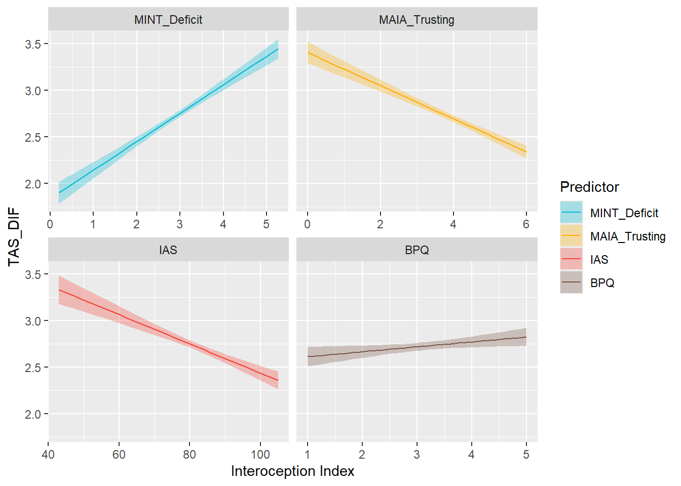
mods_dif <- compare_models_lm("TAS_DIF")
display_models(mods_dif, title="Best Model", subtitle = "DIF")preds_ddf <- compare_predictors("TAS_DDF")
display_models(preds_ddf$table, title="Best Predictor", subtitle = "DDF")preds_ddf$p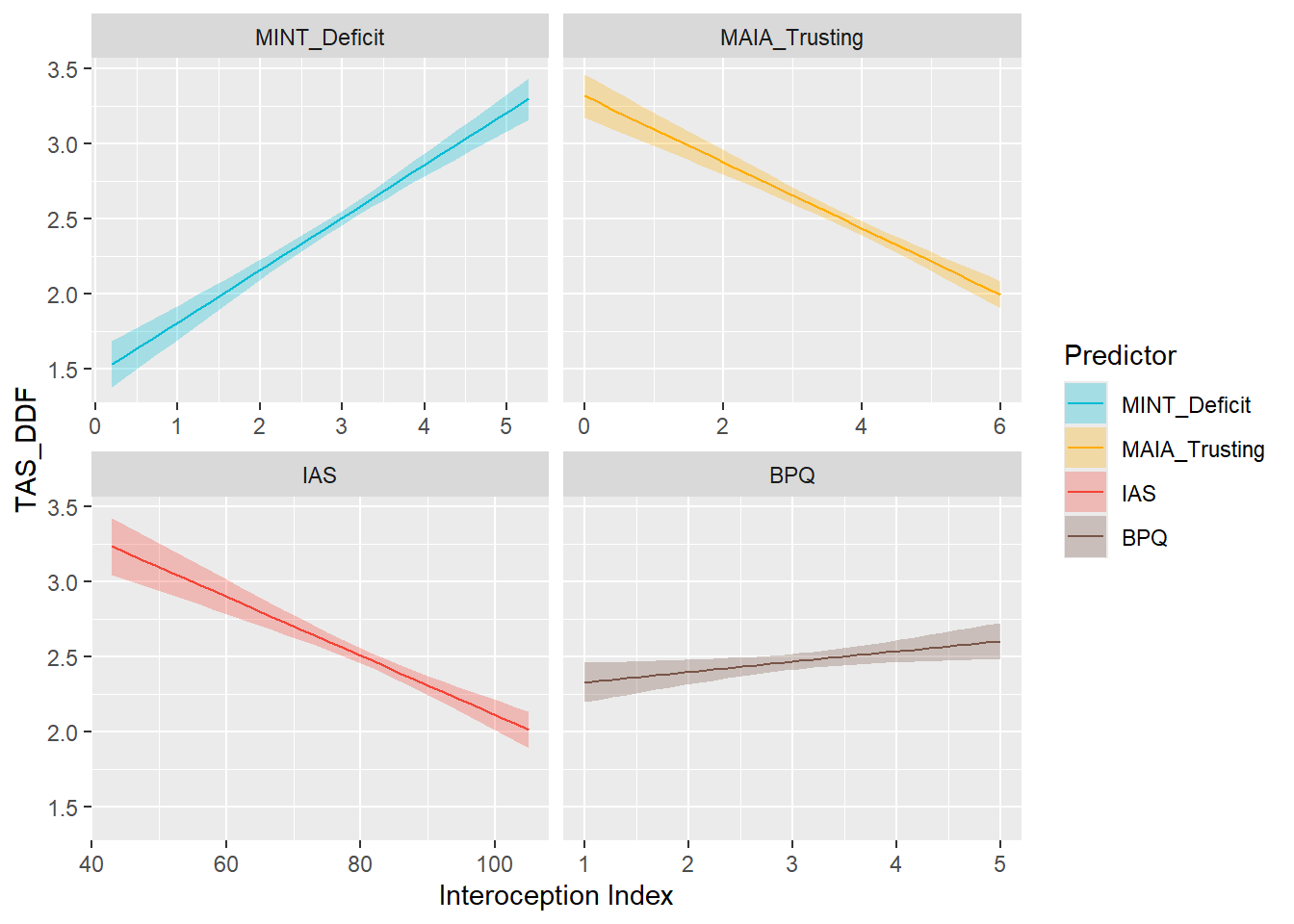
mods_ddf <- compare_models_lm("TAS_DDF")
display_models(mods_ddf, title="Best Model", subtitle = "DDF")preds_eot <- compare_predictors("TAS_EOT")
display_models(preds_eot$table, title="Best Predictor", subtitle = "EOT")preds_eot$p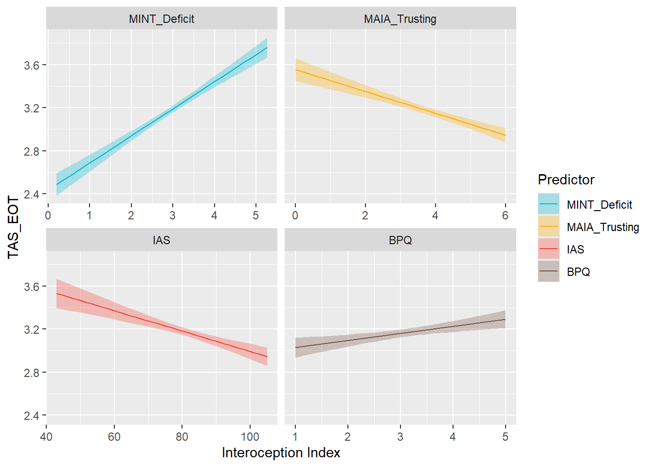
mods_eot <- compare_models_lm("TAS_EOT")
display_models(mods_eot, title="Best Model", subtitle = "EOT")make_cor(select(df, starts_with("TAS_")),
cbind(mint, metamint, select(df, starts_with("MAIA"), IAS, BPQ)))Warning: Vectorized input to `element_text()` is not officially supported.
ℹ Results may be unexpected or may change in future versions of ggplot2.
Vectorized input to `element_text()` is not officially supported.
ℹ Results may be unexpected or may change in future versions of ggplot2.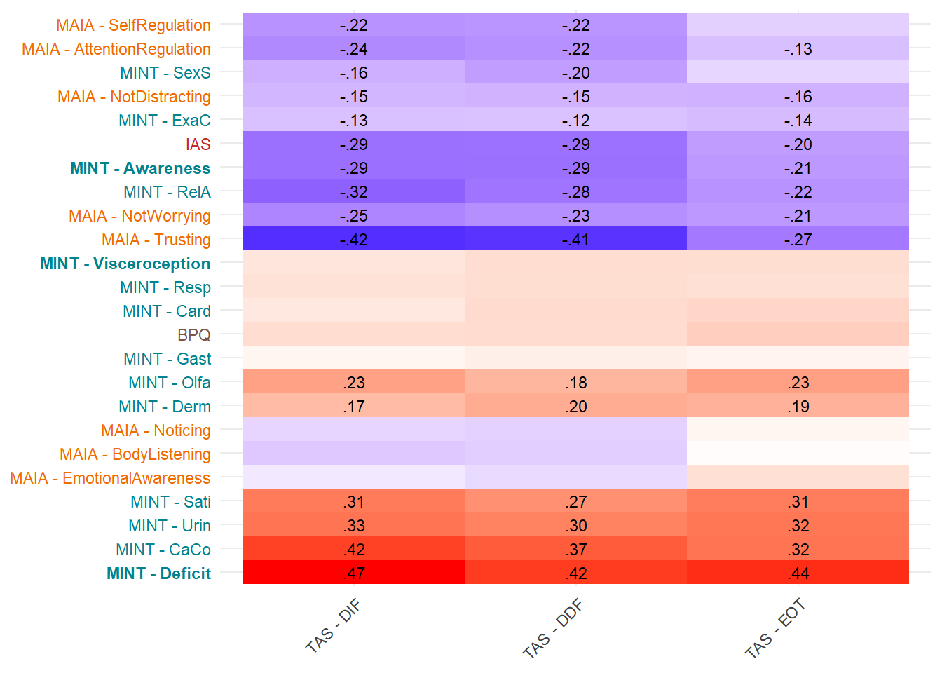
preds_ls <- compare_predictors("LifeSatisfaction")
display_models(preds_ls$table, title="Best Predictor", subtitle = "Life Satisfaction")preds_ls$p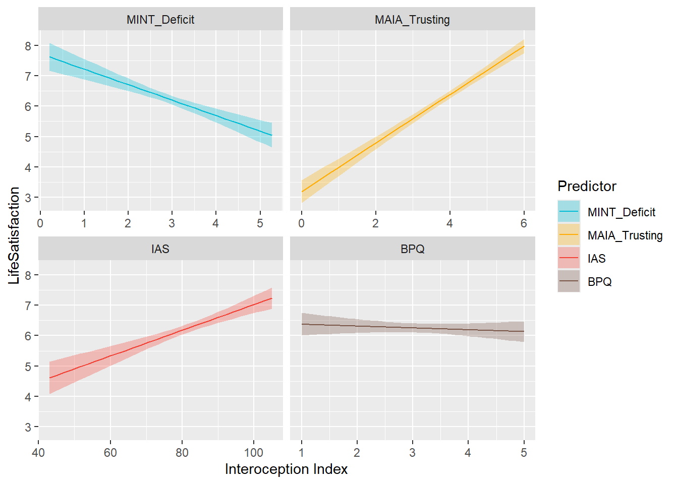
mods_ls <- compare_models_lm("LifeSatisfaction")
display_models(mods_ls, title="Best Model", subtitle = "Life Satisfaction")preds_anx <- compare_predictors("PHQ4_Anxiety")
display_models(preds_anx$table, title="Best Predictor", subtitle = "PHQ4 Anxiety")preds_anx$p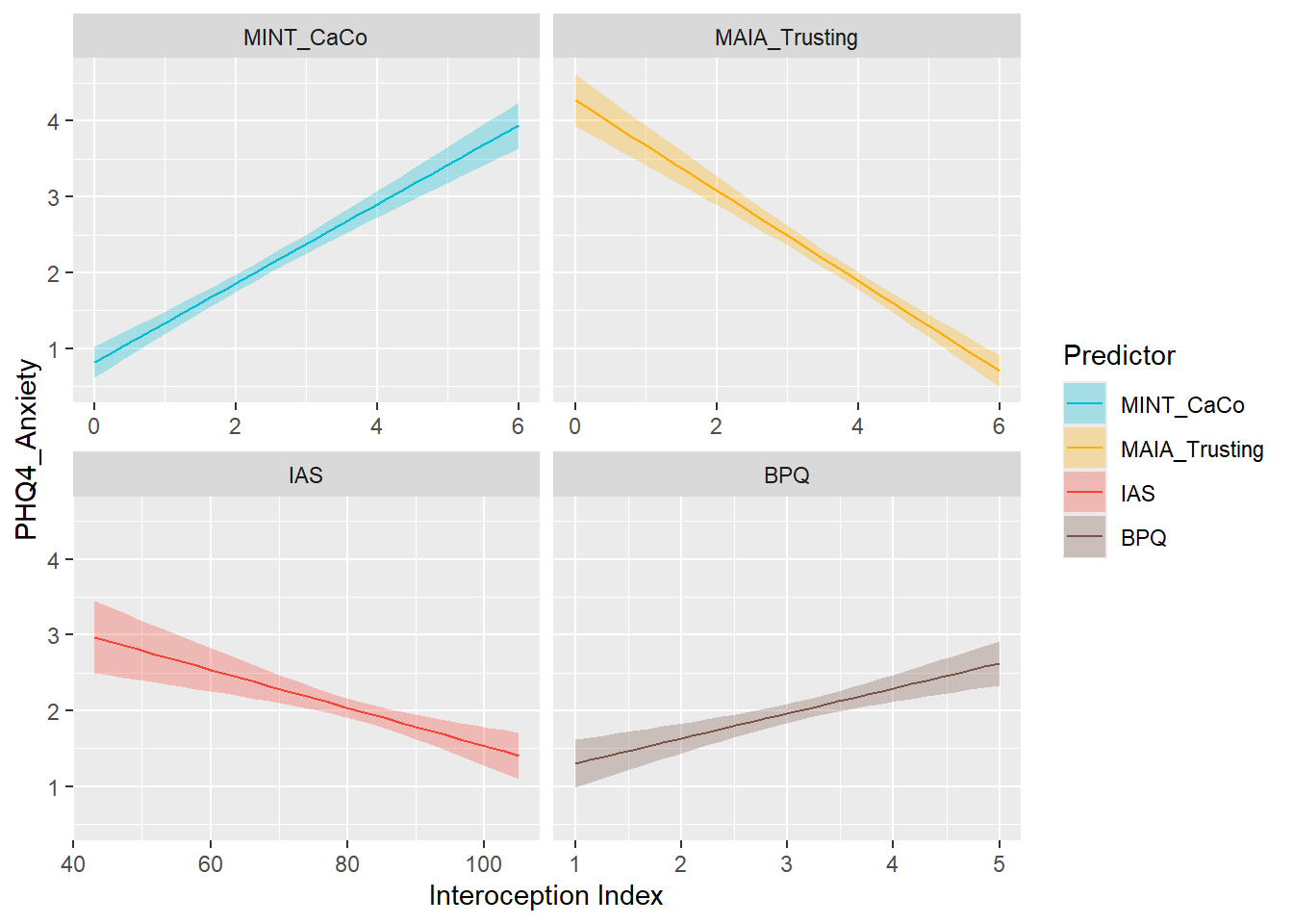
mods_anx <- compare_models_lm("PHQ4_Anxiety")
display_models(mods_anx, title="Best Model", subtitle = "PHQ4 Anxiety")preds_dep <- compare_predictors("PHQ4_Depression")
display_models(preds_dep$table, title="Best Predictor", subtitle = "PHQ4 Depression")preds_dep$p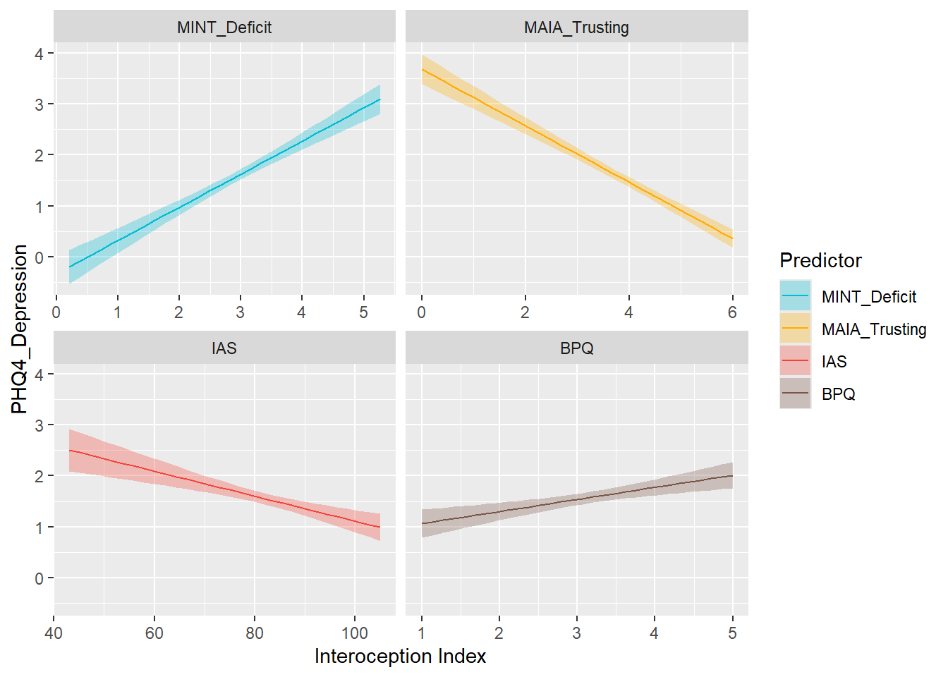
mods_dep <- compare_models_lm("PHQ4_Depression")
display_models(mods_dep, title="Best Model", subtitle = "PHQ4 Depression")make_cor(select(df, LifeSatisfaction, starts_with("PHQ4_")),
cbind(mint, metamint, select(df, starts_with("MAIA"), IAS, BPQ)))Warning: Vectorized input to `element_text()` is not officially supported.
ℹ Results may be unexpected or may change in future versions of ggplot2.
Vectorized input to `element_text()` is not officially supported.
ℹ Results may be unexpected or may change in future versions of ggplot2.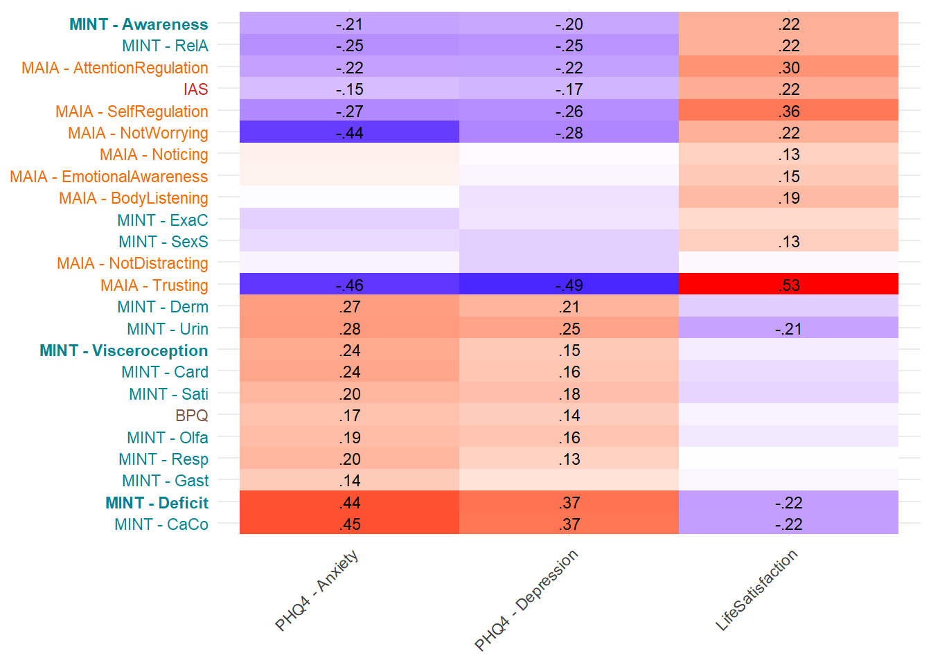
preds_arou <- compare_predictors("ERS_Arousal")
display_models(preds_arou$table, title="Best Predictor", subtitle = "ERS Arousal")preds_arou$p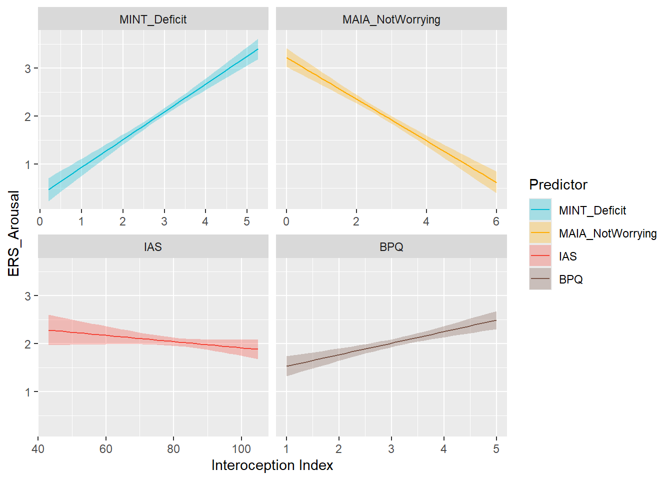
mods_arou <- compare_models_lm("ERS_Arousal")
display_models(mods_arou, title="Best Model", subtitle = "ERS Arousal")preds_sens <- compare_predictors("ERS_Sensitivity")
display_models(preds_sens$table, title="Best Predictor", subtitle = "ERS Sensitivity")preds_sens$p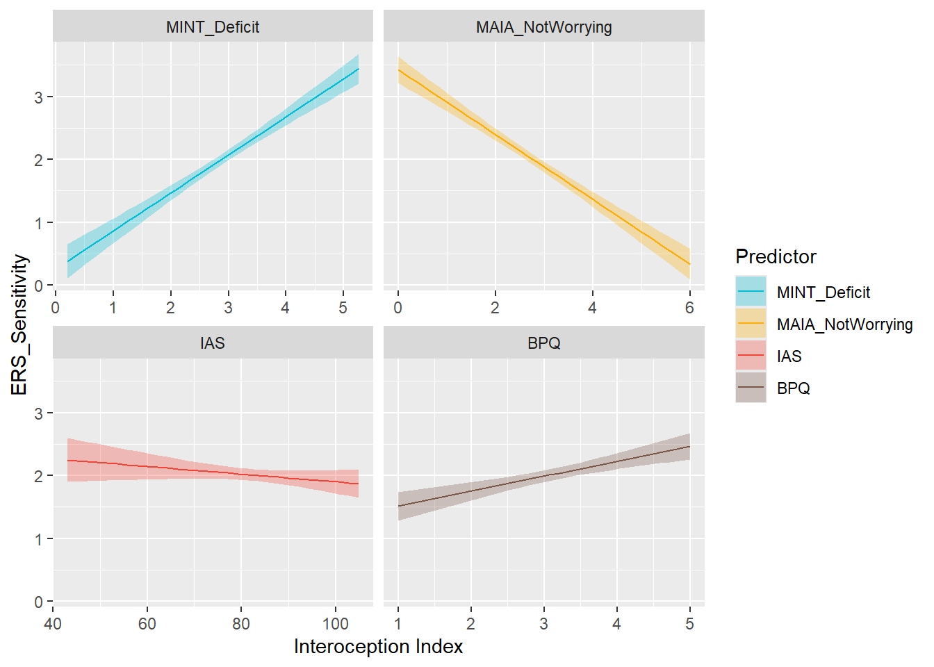
mods_sens <- compare_models_lm("ERS_Sensitivity")
display_models(mods_sens, title="Best Model", subtitle = "ERS Sensitivity")preds_pers <- compare_predictors("ERS_Persistence")
display_models(preds_pers$table, title="Best Predictor", subtitle = "ERS Persistence")preds_pers$p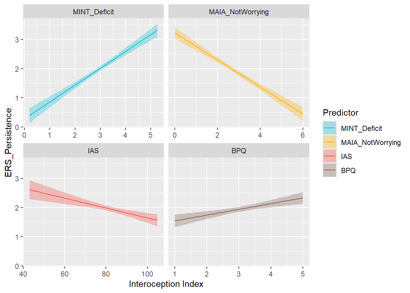
mods_pers <- compare_models_lm("ERS_Persistence")
display_models(mods_pers, title="Best Model", subtitle = "ERS Persistence")make_cor(select(df, starts_with("ERS_")),
cbind(mint, metamint, select(df, starts_with("MAIA"), IAS, BPQ)))Warning: Vectorized input to `element_text()` is not officially supported.
ℹ Results may be unexpected or may change in future versions of ggplot2.
Vectorized input to `element_text()` is not officially supported.
ℹ Results may be unexpected or may change in future versions of ggplot2.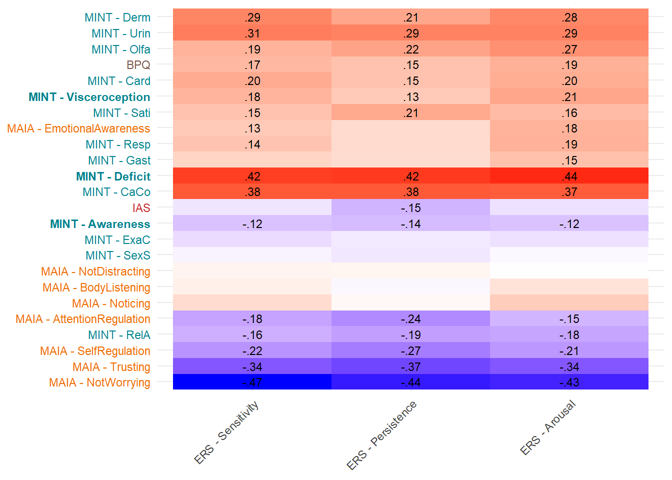
make_cor(select(df, starts_with("CEFSA")),
cbind(mint, metamint, select(df, starts_with("MAIA"), IAS, BPQ)))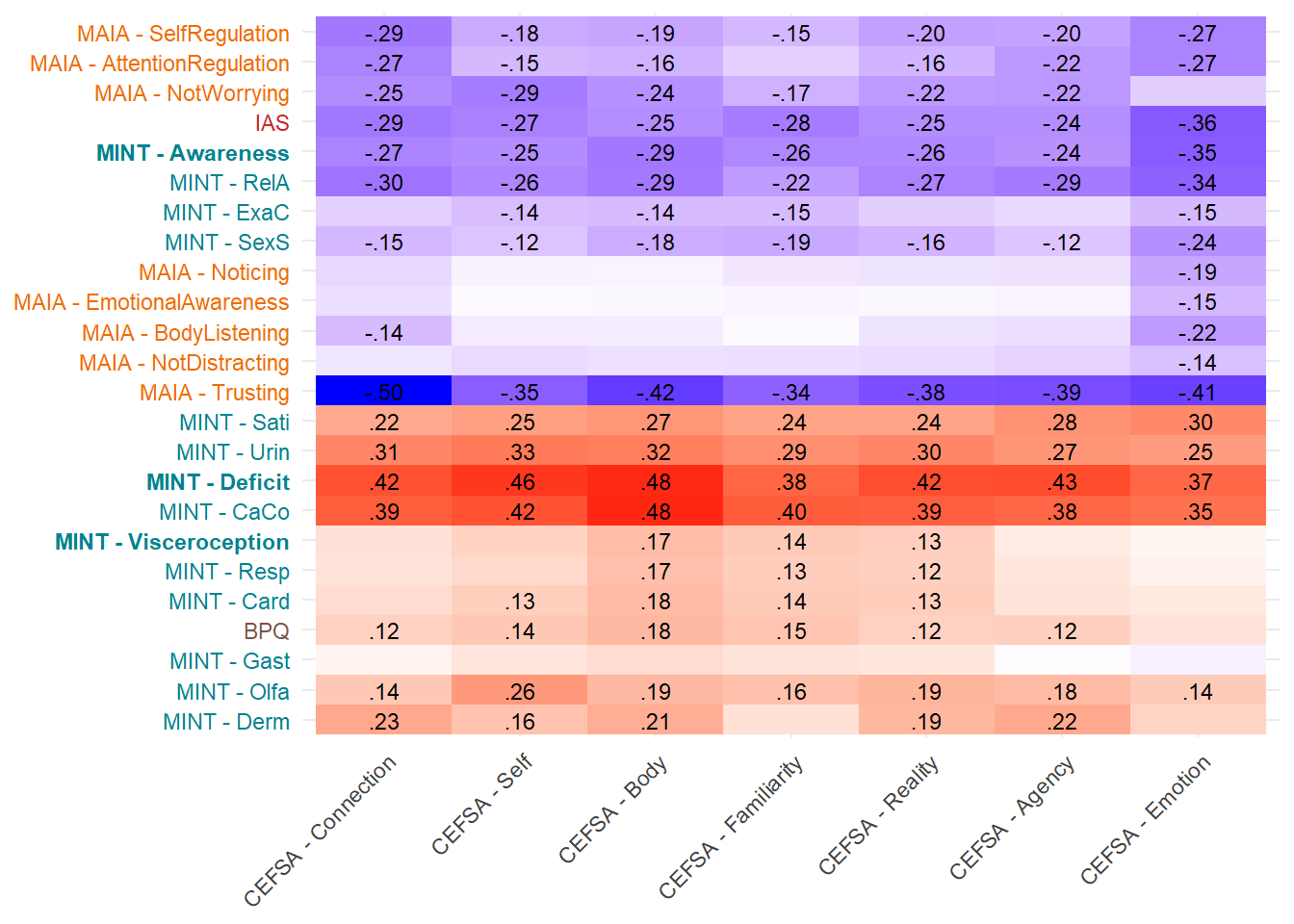
preds_cefsabody <- compare_predictors("CEFSA_Body")
display_models(preds_cefsabody$table, title="Best Predictor", subtitle = "CEFSA - Body")preds_cefsabody$p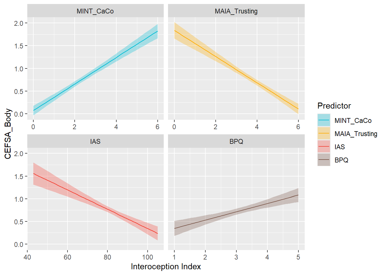
mods_cefsabody <- compare_models_lm("CEFSA_Body")
display_models(mods_cefsabody, title="Best Model", subtitle = "CEFSA - Body")preds_cefsaself <- compare_predictors("CEFSA_Self")
display_models(preds_cefsaself$table, title="Best Predictor", subtitle = "CEFSA - Self")preds_cefsaself$p
mods_cefsaself <- compare_models_lm("CEFSA_Self")
display_models(mods_cefsaself, title="Best Model", subtitle = "CEFSA - Self")preds_cefsaemo <- compare_predictors("CEFSA_Emotion")
display_models(preds_cefsaemo$table, title="Best Predictor", subtitle = "CEFSA - Emotion")preds_cefsaemo$p
mods_cefsaemo <- compare_models_lm("CEFSA_Emotion")
display_models(mods_cefsaemo, title="Best Model", subtitle = "CEFSA - Emotion")preds_cefsareal <- compare_predictors("CEFSA_Reality")
display_models(preds_cefsareal$table, title="Best Predictor", subtitle = "CEFSA - Reality")preds_cefsareal$p
mods_cefsareal <- compare_models_lm("CEFSA_Reality")
display_models(mods_cefsareal, title="Best Model", subtitle = "CEFSA - Reality")preds_cefsacon <- compare_predictors("CEFSA_Connection")
display_models(preds_cefsacon$table, title="Best Predictor", subtitle = "CEFSA - Connection")preds_cefsacon$p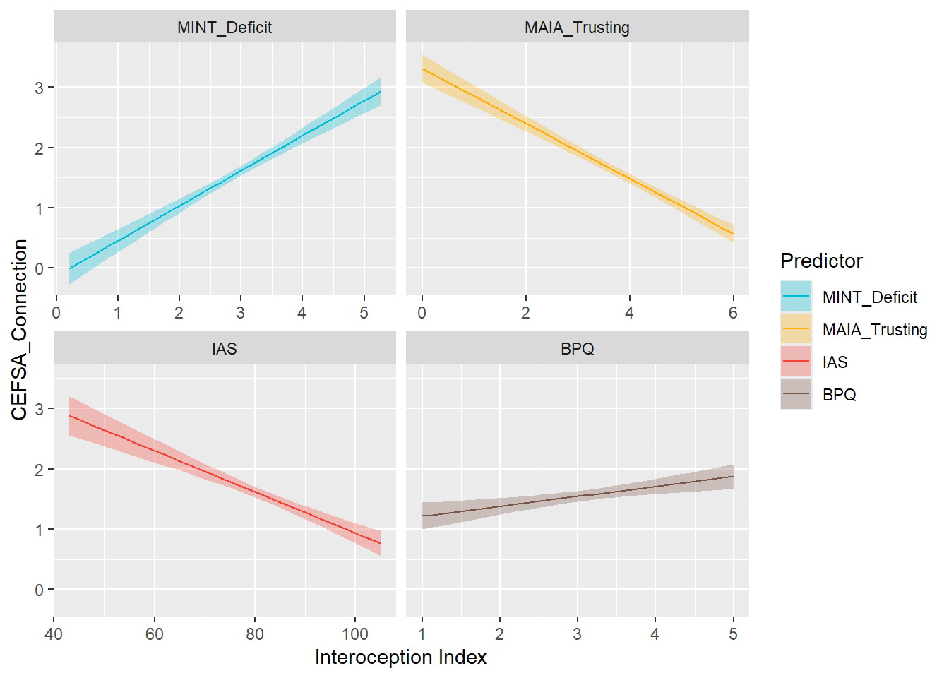
mods_cefsacon <- compare_models_lm("CEFSA_Connection")
display_models(mods_cefsacon, title="Best Model", subtitle = "CEFSA - Connection")preds_cefsagency <- compare_predictors("CEFSA_Agency")
display_models(preds_cefsagency$table, title="Best Predictor", subtitle = "CEFSA - Agency")preds_cefsagency$p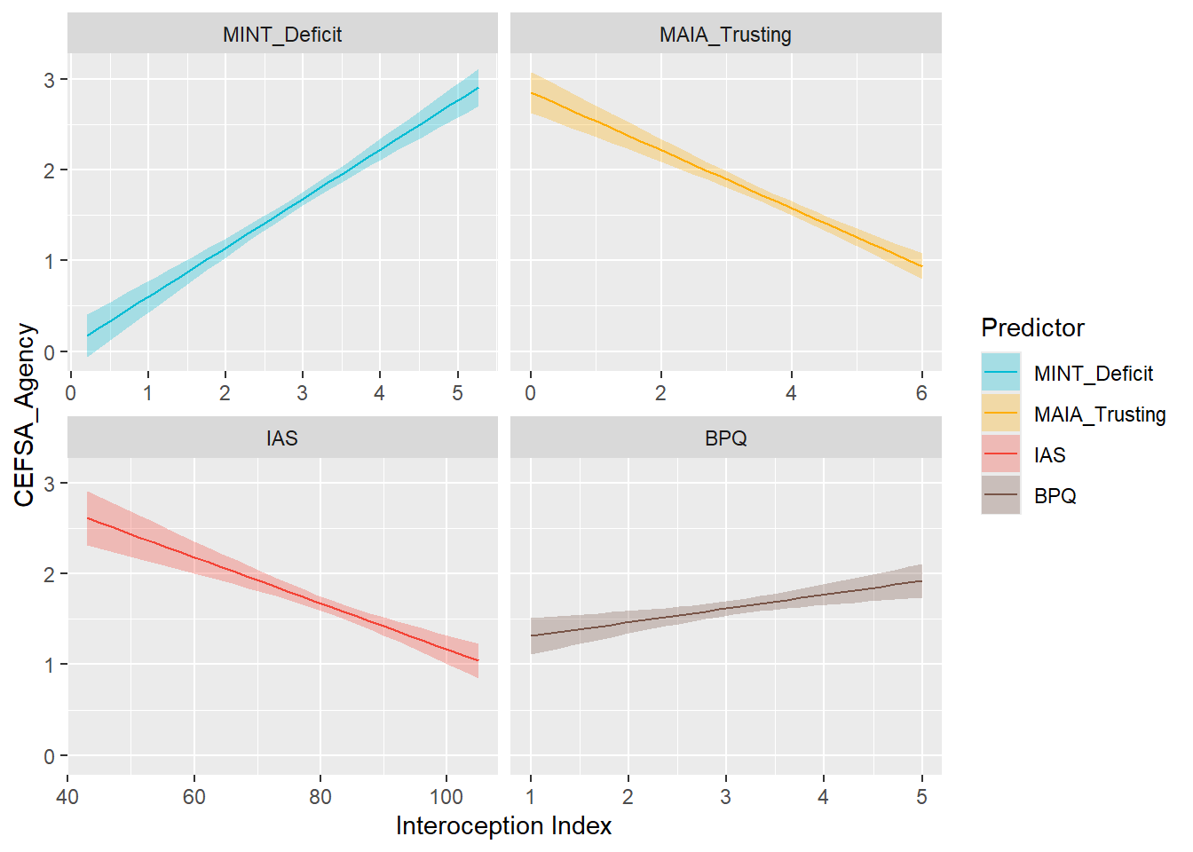
mods_cefsagency <- compare_models_lm("CEFSA_Agency")
display_models(mods_cefsagency, title="Best Model", subtitle = "CEFSA - Agency")make_cor(select(df, starts_with("CERQ")),
cbind(mint, metamint, select(df, starts_with("MAIA"), IAS, BPQ)))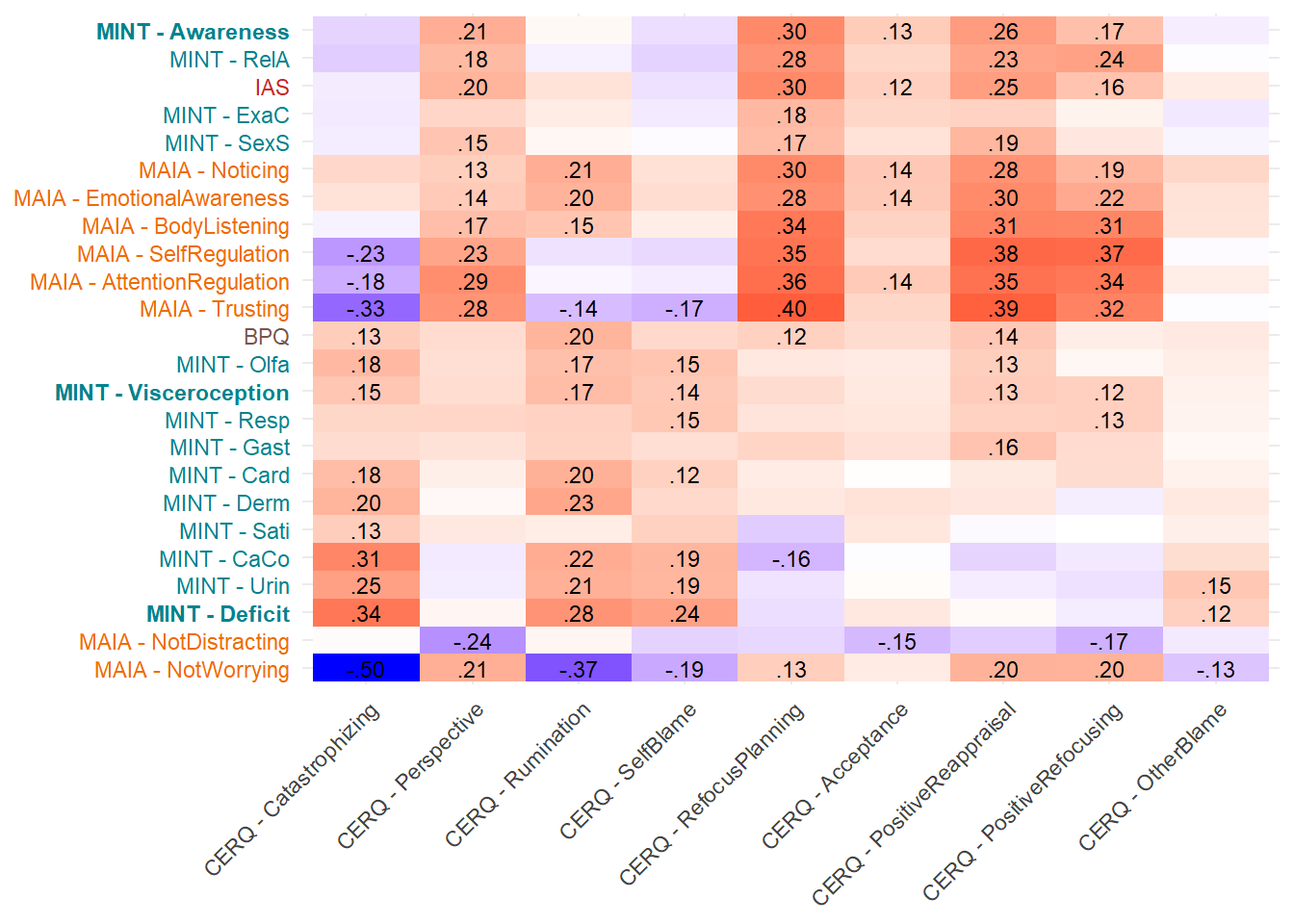
preds_cerqreapp <- compare_predictors("CERQ_PositiveReappraisal")
display_models(preds_cerqreapp$table, title="Best Predictor", subtitle = "CERQ - Positive Reappraisal")preds_cerqreapp$p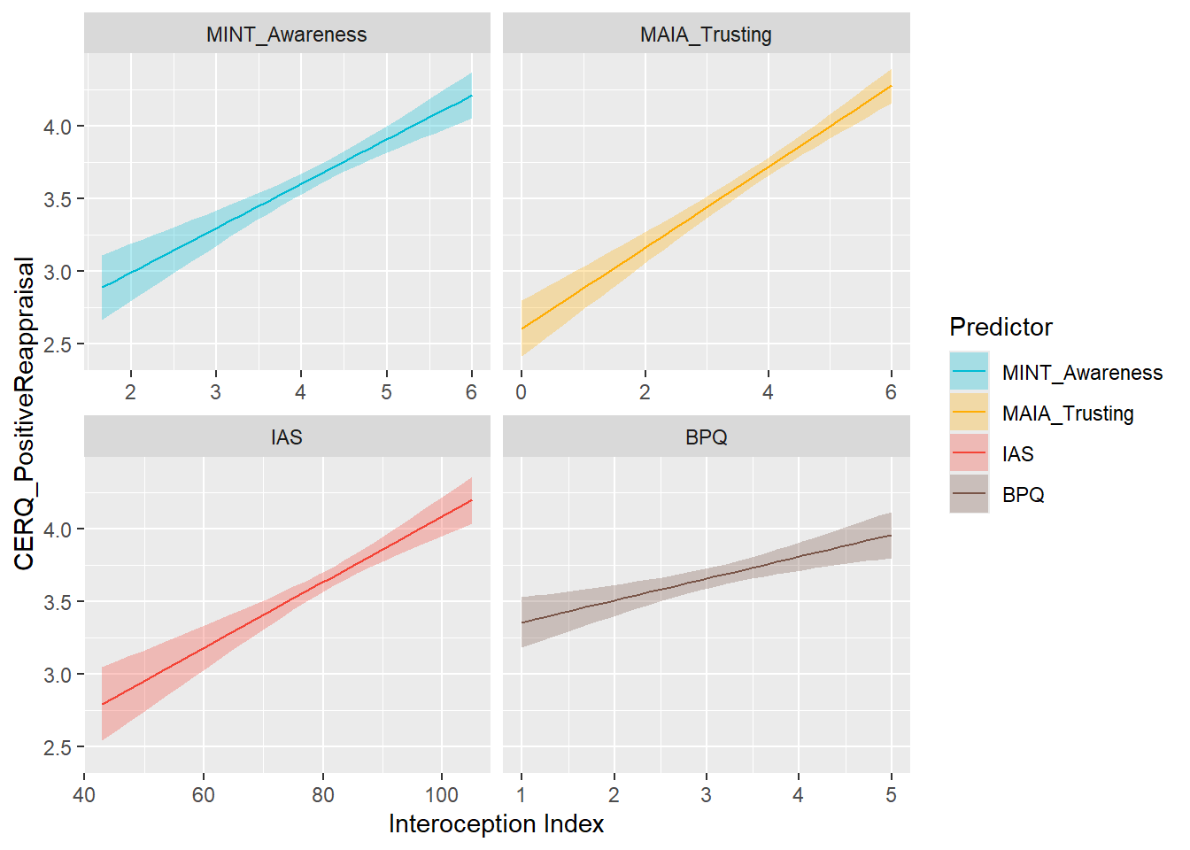
mods_cerqreapp <- compare_models_lm("CERQ_PositiveReappraisal")
display_models(mods_cerqreapp, title="Best Model", subtitle = "CERQ - Positive Reappraisal")preds_cerqrefocus <- compare_predictors("CERQ_PositiveRefocusing")
display_models(preds_cerqrefocus$table, title="Best Predictor", subtitle = "CERQ - Positive Refocusing")preds_cerqrefocus$p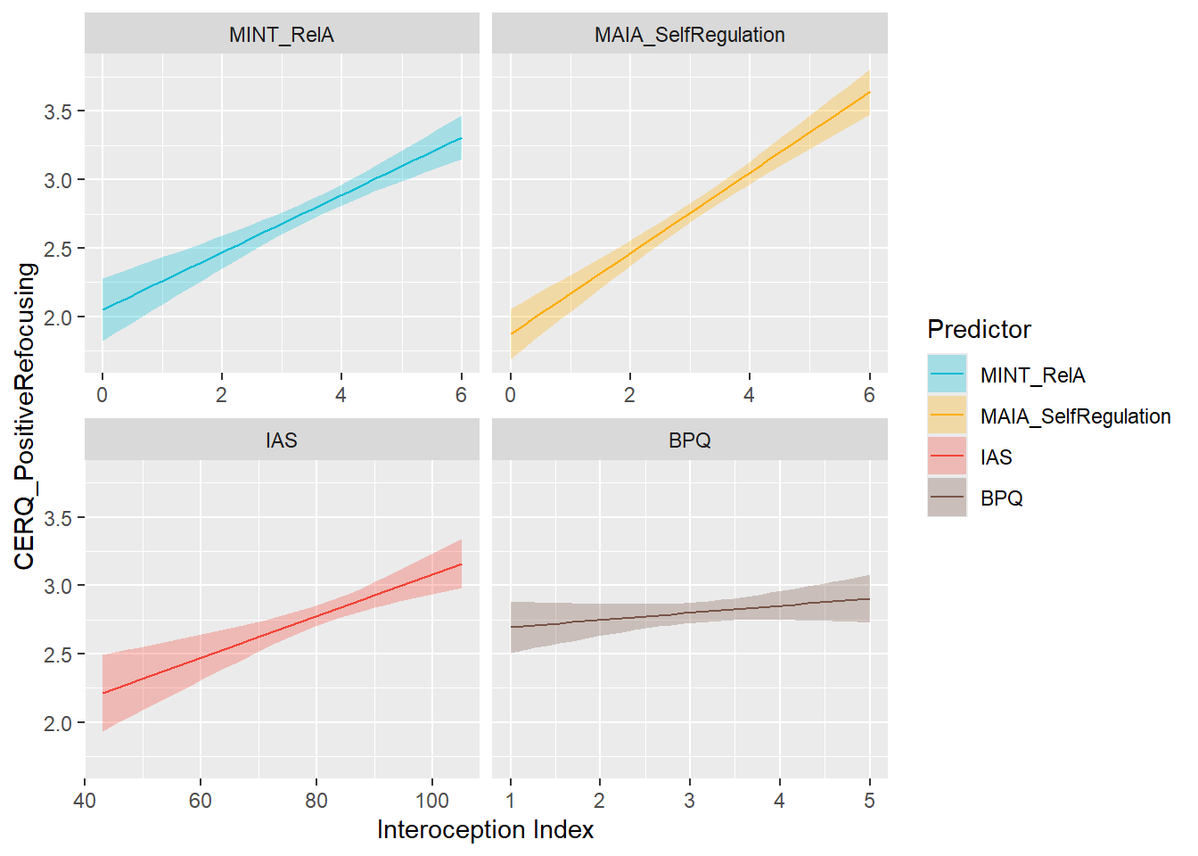
mods_cerqrefocus <- compare_models_lm("CERQ_PositiveRefocusing")
display_models(mods_cerqrefocus, title="Best Model", subtitle = "CERQ - Positive Refocusing")preds_cerqpersp <- compare_predictors("CERQ_Perspective")
display_models(preds_cerqpersp$table, title="Best Predictor", subtitle = "CERQ - Perspective")preds_cerqpersp$p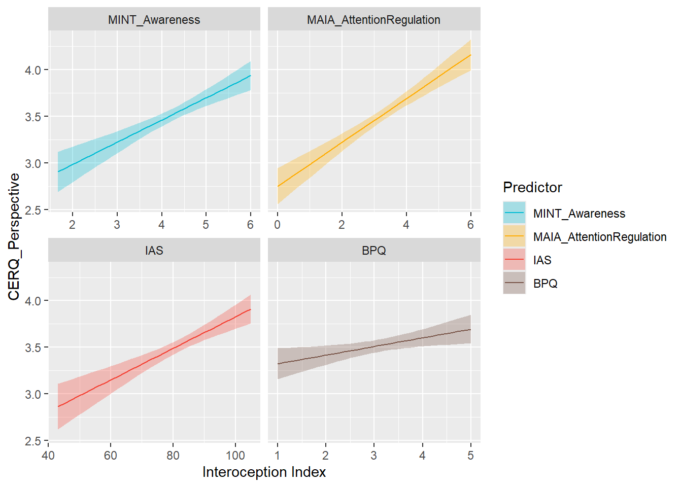
mods_cerqpersp <- compare_models_lm("CERQ_Perspective")
display_models(mods_cerqpersp, title="Best Model", subtitle = "CERQ - Perspective")preds_cerqacceptance <- compare_predictors("CERQ_Acceptance")
display_models(preds_cerqacceptance$table, title="Best Predictor", subtitle = "CERQ - Acceptance")preds_cerqacceptance$p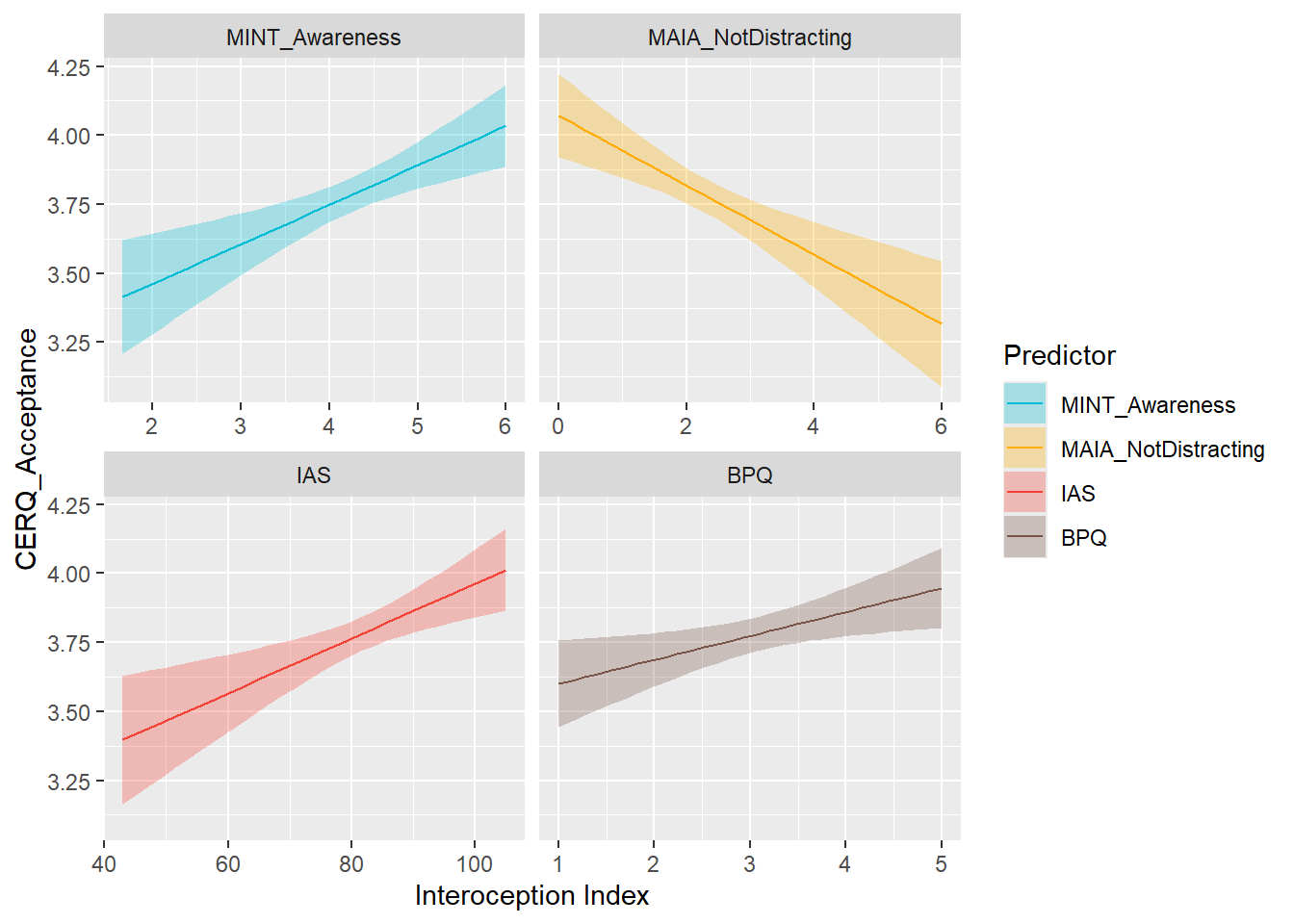
mods_cerqacceptance <- compare_models_lm("CERQ_Acceptance")
display_models(mods_cerqacceptance, title="Best Model", subtitle = "CERQ - Acceptance")make_cor(select(df, starts_with("PI")),
cbind(mint, metamint, select(df, starts_with("MAIA"), IAS, BPQ)))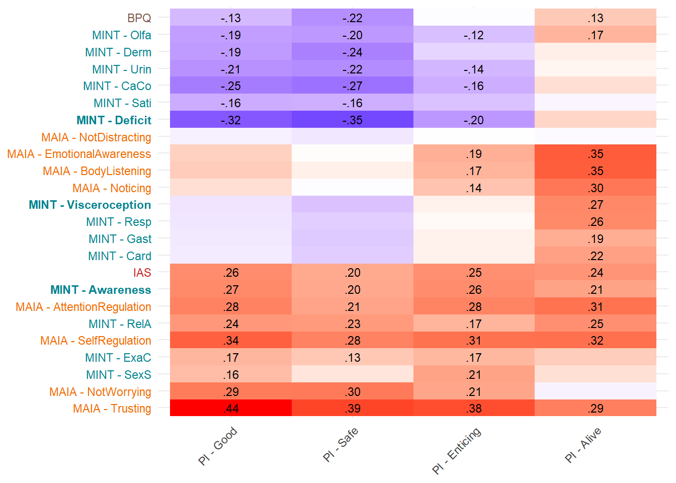
preds_pialive <- compare_predictors("PI_Alive")
display_models(preds_pialive$table, title="Best Predictor", subtitle = "Primals - Alive")preds_pialive$p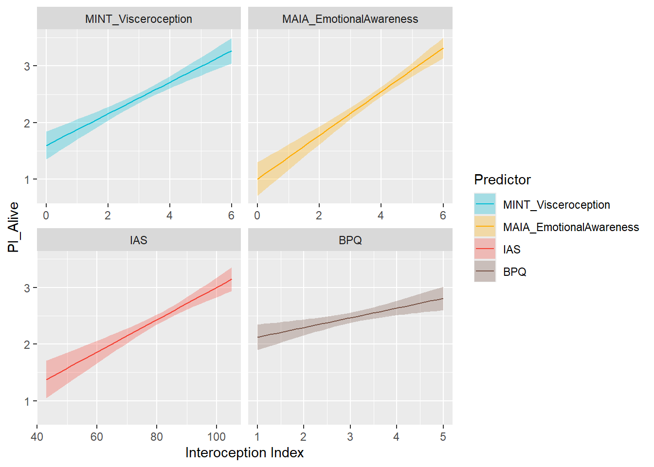
mods_pialive <- compare_models_lm("PI_Alive")
display_models(mods_pialive, title="Best Model", subtitle = "Primals - Alive")preds_pisafe <- compare_predictors("PI_Safe")
display_models(preds_pisafe$table, title="Best Predictor", subtitle = "Primals - Safe")preds_pisafe$p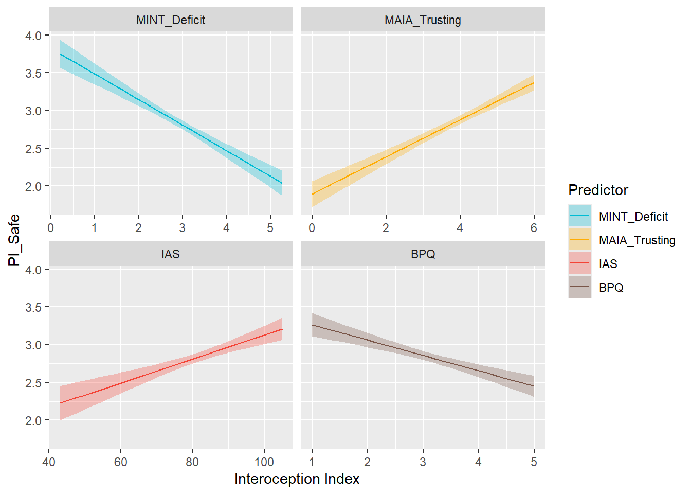
mods_pisafe <- compare_models_lm("PI_Safe")
display_models(mods_pisafe, title="Best Model", subtitle = "Primals - Safe")preds_pient <- compare_predictors("PI_Enticing")
display_models(preds_pient$table, title="Best Predictor", subtitle = "Primals - Enticing")preds_pient$p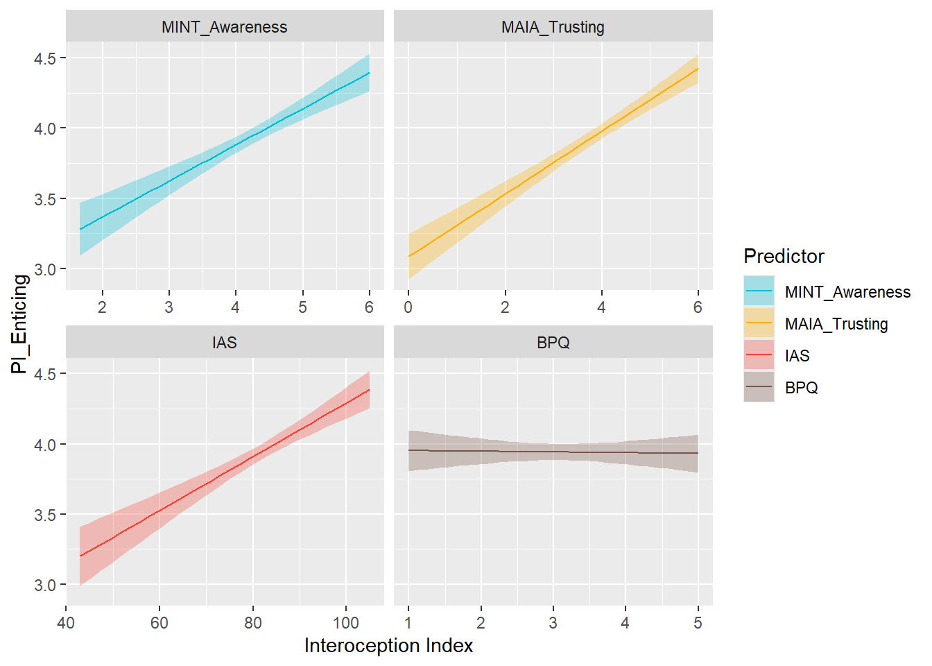
mods_pient <- compare_models_lm("PI_Enticing")
display_models(mods_pient, title="Best Model", subtitle = "Primals - Enticing")preds_pigood <- compare_predictors("PI_Good")
display_models(preds_pigood$table, title="Best Predictor", subtitle = "Primals - Good")preds_pigood$p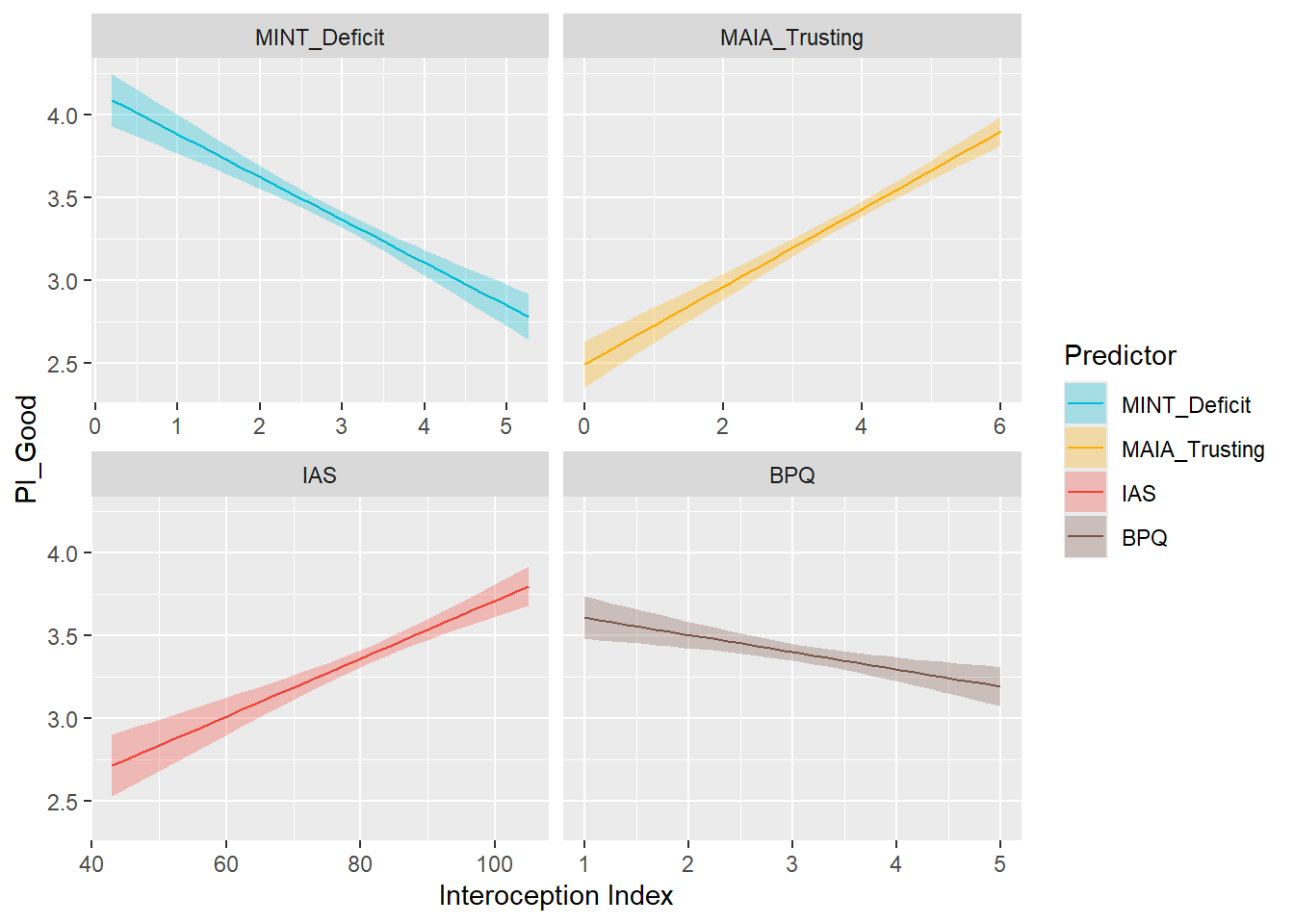
mods_pigood <- compare_models_lm("PI_Good")
display_models(mods_pigood, title="Best Model", subtitle = "Primals - Good")compare_models_glm <- function(outcome="Disorders_Psychiatric_Mood", title="", subtitle = "") {
# Full Questionnaires
m_mint <- glm(as.formula(paste0(outcome, " ~ .")),
data = cbind(mint, df[outcome]),
family = "binomial")
m_metamint <- glm(as.formula(paste0(outcome, " ~ .")),
data = cbind(metamint, df[outcome]),
family = "binomial")
m_minimint <- glm(as.formula(paste0(outcome, " ~ .")),
data = cbind(minimint, df[outcome]),
family = "binomial")
m_micromint <- glm(as.formula(paste0(outcome, " ~ .")),
data = cbind(micromint, df[outcome]),
family = "binomial")
m_ias <- glm(as.formula(paste0(outcome, " ~ IAS")),
data = df,
family = "binomial")
m_maia <- glm(as.formula(paste0(outcome, " ~ .")),
data = select(df, all_of(outcome), starts_with("MAIA")),
family = "binomial")
m_imaia <- glm(as.formula(paste0(outcome, " ~ .")),
data = select(df, all_of(outcome),
# MAIA_AttentionRegulation, # remove?
# MAIA_SelfRegulation, # remove?
# MAIA_Trusting, # remove?
MAIA_BodyListening,
MAIA_EmotionalAwareness,
MAIA_Noticing),
family = "binomial")
m_bpq <- glm(as.formula(paste0(outcome, " ~ BPQ")),
data = df,
family = "binomial")
models_full <- list(m_mint=m_mint, m_metamint=m_metamint,
m_minimint=m_minimint, m_micromint=m_micromint,
m_maia=m_maia, m_imaia=m_imaia,
m_ias=m_ias, m_bpq=m_bpq)
table <- table_models(models_full)
get_auc <- function(m) {
roc <- as.data.frame(performance_roc(m))
auc <- bayestestR::area_under_curve(roc$Specificity, roc$Sensitivity)
paste0("AUC = ", insight::format_percent(auc))
}
mods_order <- c("Mint", "metaMint", "miniMint", "microMint", "MAIA", "iMAIA", "IAS", "BPQ")
p <- rbind(
mutate(as.data.frame(performance_roc(m_mint)), Predictor = "Mint"),
mutate(as.data.frame(performance_roc(m_metamint)), Predictor = "metaMint"),
mutate(as.data.frame(performance_roc(m_minimint)), Predictor = "miniMint"),
mutate(as.data.frame(performance_roc(m_micromint)), Predictor = "microMint"),
mutate(as.data.frame(performance_roc(m_maia)), Predictor = "MAIA"),
mutate(as.data.frame(performance_roc(m_imaia)), Predictor = "iMAIA"),
mutate(as.data.frame(performance_roc(m_ias)), Predictor = "IAS"),
mutate(as.data.frame(performance_roc(m_bpq)), Predictor = "BPQ")
) |>
mutate(Predictor = fct_relevel(Predictor, mods_order)) |>
ggplot(aes(x=Specificity)) +
geom_abline(intercept=0, slope=1, color="gray", linewidth=1) +
geom_line(aes(y=Sensitivity, color=Predictor), linewidth=1.5, alpha=0.9) +
geom_label(data=data.frame(
label = c(get_auc(m_mint), get_auc(m_metamint),
get_auc(m_minimint), get_auc(m_micromint),
get_auc(m_maia), get_auc(m_imaia), get_auc(m_ias), get_auc(m_bpq)),
Predictor = mods_order,
x = 0.8,
y = c(0.55, 0.475, 0.425, 0.375, 0.30, 0.25, 0.20, 0.15)),
aes(x=x, y=y, label=label), color=colors[mods_order], size=3) +
labs(x= "1 - Specificity (False Positive Rate)", y="Sensitivity (True Positive Rate)",
color="Questionnaire", title = title, subtitle=subtitle) +
scale_color_manual(values=colors) +
scale_x_continuous(labels=scales::percent) +
scale_y_continuous(labels=scales::percent) +
theme_minimal() +
theme(plot.title = element_text(face="bold"))
list(table=table, p=p)
}preds_mood <- compare_predictors("Disorders_Psychiatric_Mood")
display_models(preds_mood$table, title="Best Predictor", subtitle = "Mood Disorders")preds_mood$p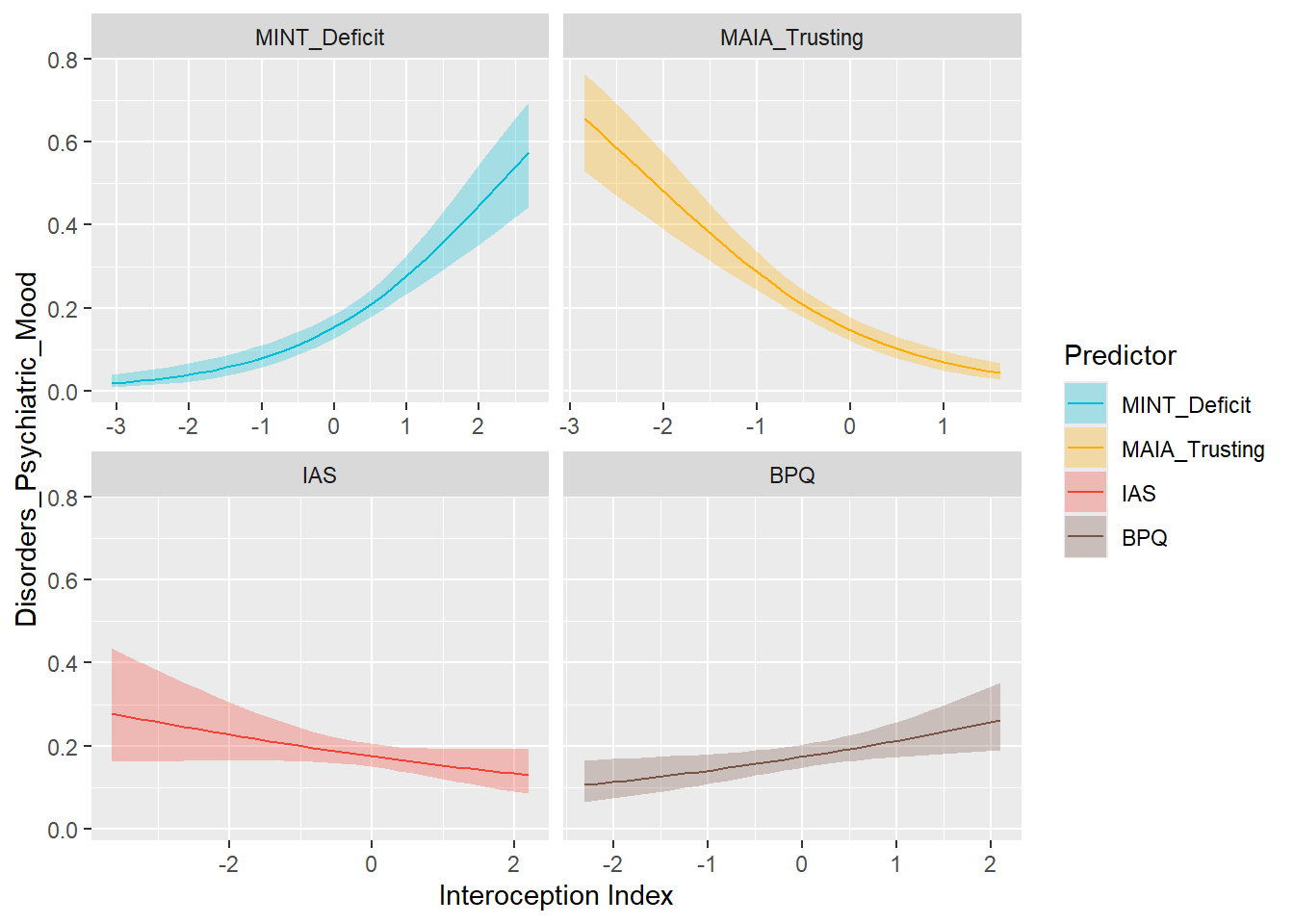
mods_mood <- compare_models_glm("Disorders_Psychiatric_Mood")
display_models(mods_mood$table, title="Best Predictor", subtitle = "Mood Disorders")mods_mood$p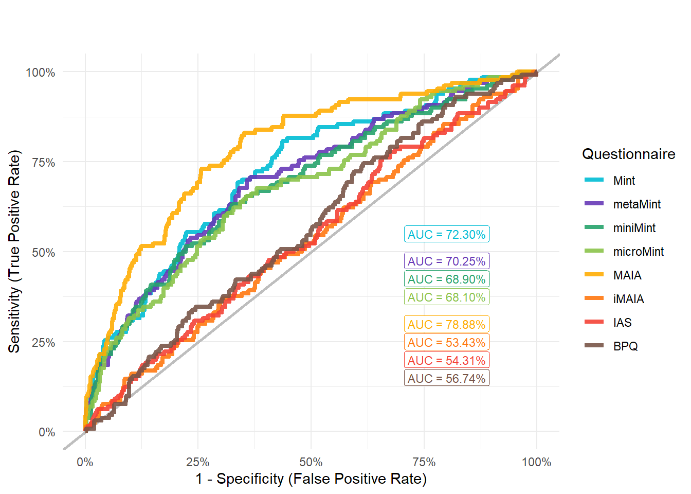
preds_moodt <- compare_predictors("Disorders_Psychiatric_MoodTreatment")
display_models(preds_moodt$table, title="Best Predictor", subtitle = "Mood Disorders (with Treatment)")preds_moodt$p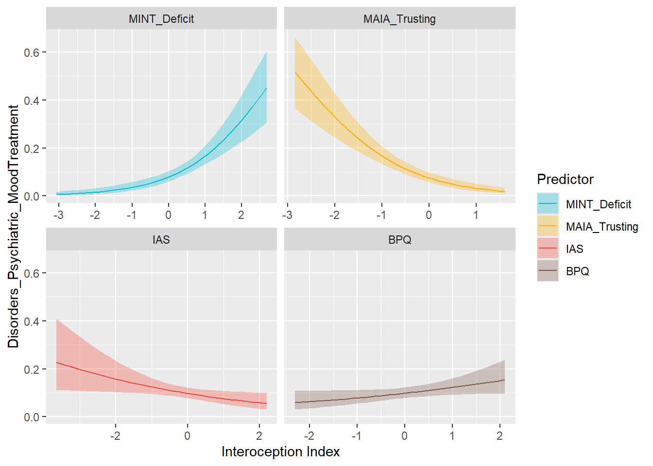
mods_moodt <- compare_models_glm("Disorders_Psychiatric_MoodTreatment",
title="Mood Disorders", subtitle = "MDD, GAD, Bipolar (with Treatment)")
display_models(mods_moodt$table, title="Best Predictor", subtitle = "Mood Disorders (with Treatment)")mods_moodt$p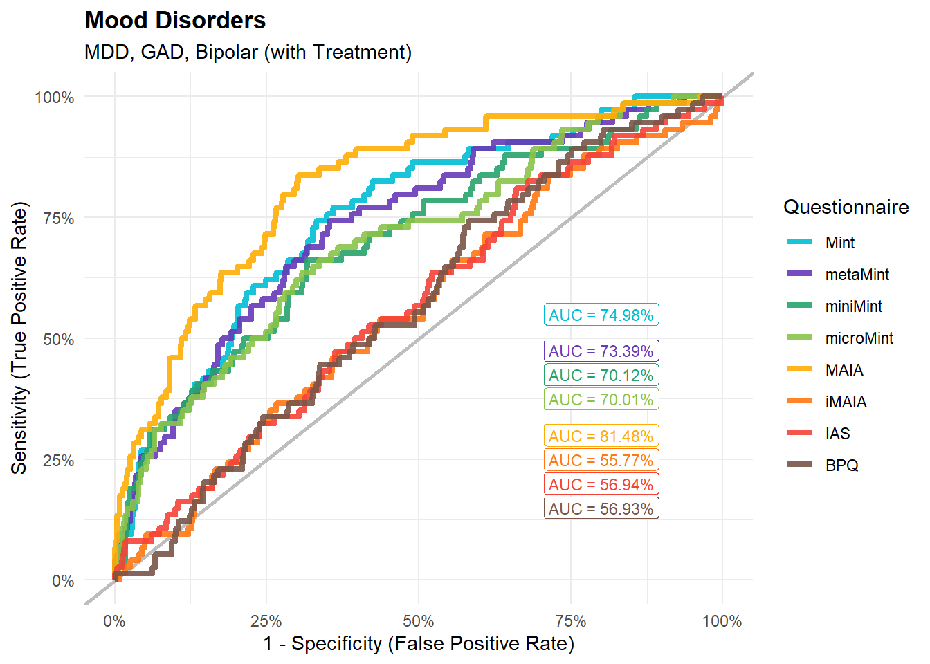
preds_anxdis <- compare_predictors("Disorders_Psychiatric_Anxiety")
display_models(preds_anxdis$table, title="Best Predictor", subtitle = "Anxiety Disorders")preds_anxdis$p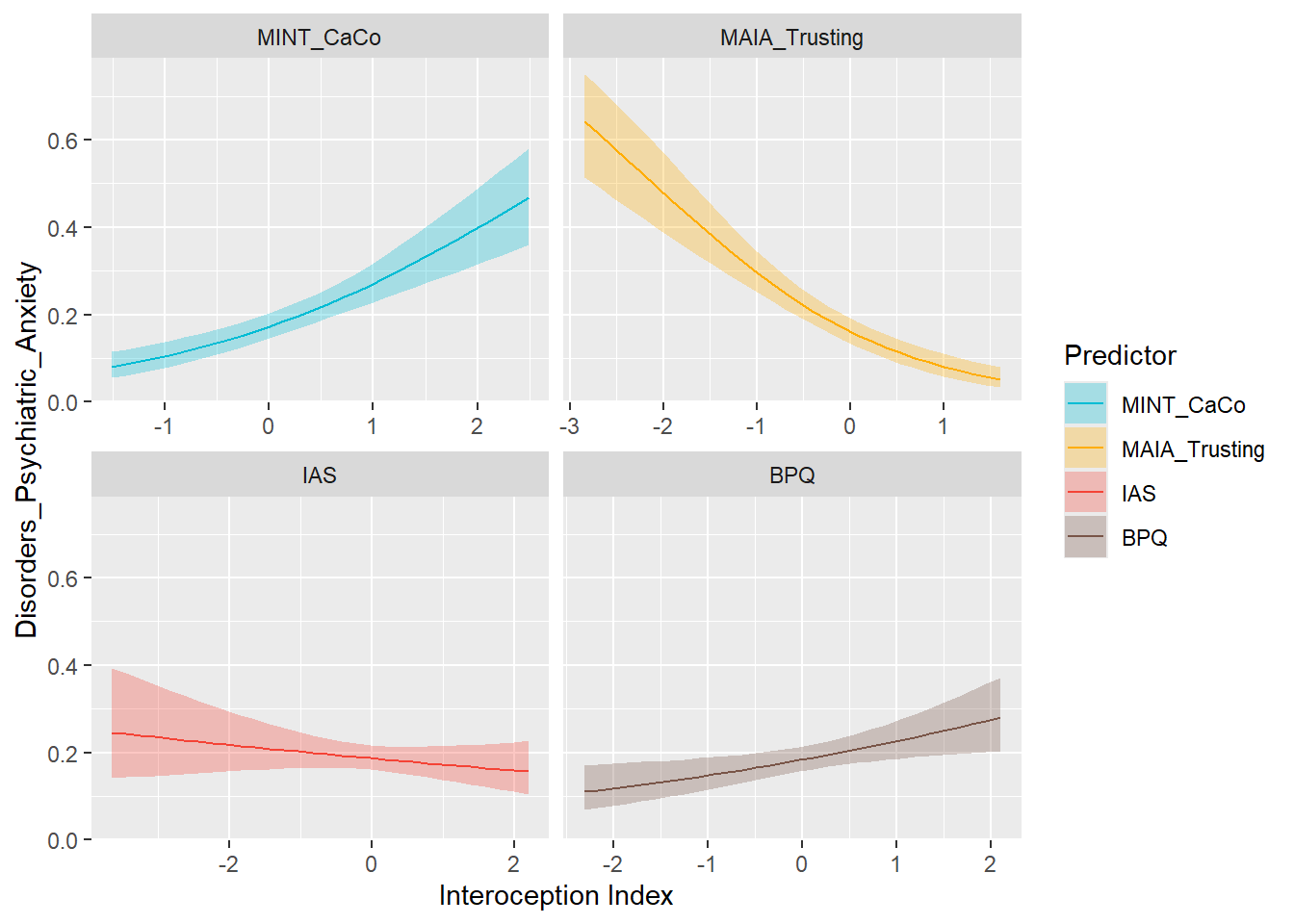
mods_anxdis <- compare_models_glm("Disorders_Psychiatric_Anxiety")
display_models(mods_anxdis$table, title="Best Model", subtitle = "Anxiety Disorders")mods_anxdis$p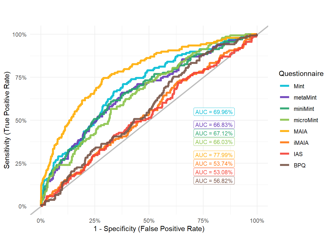
preds_anxdist <- compare_predictors("Disorders_Psychiatric_AnxietyTreatment")
display_models(preds_anxdist$table, title="Best Predictor", subtitle = "Anxiety Disorders (with Treatment)")preds_anxdist$p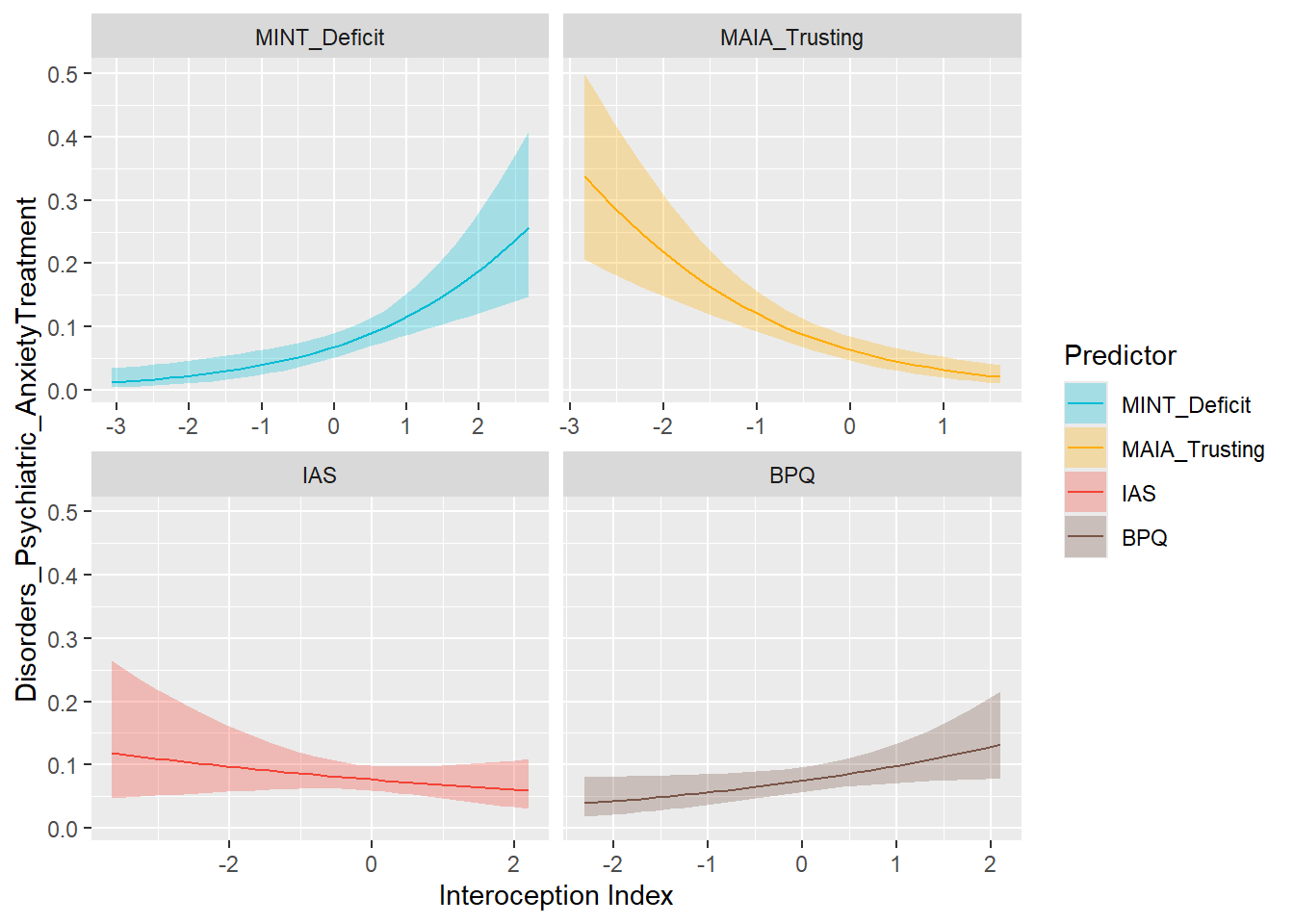
mods_anxdist <- compare_models_glm("Disorders_Psychiatric_AnxietyTreatment")
display_models(mods_anxdist$table, title="Best Model", subtitle = "Anxiety Disorders (with Treatment)")mods_anxdist$p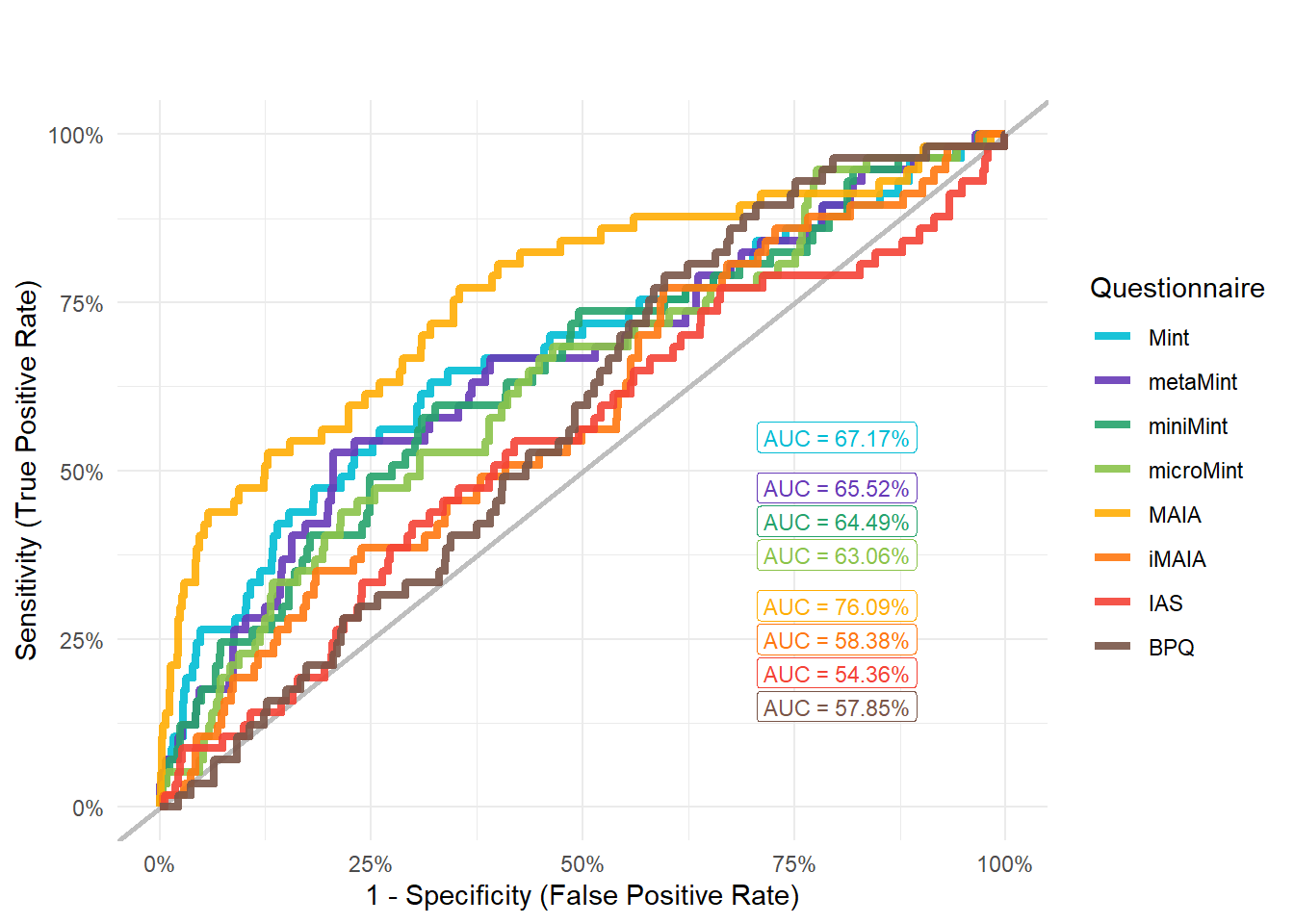
preds_eat <- compare_predictors("Disorders_Psychiatric_Eating")
display_models(preds_eat$table, title="Best Predictor", subtitle = "Eating Disorders")preds_eat$p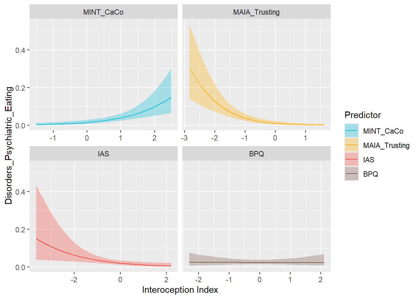
mods_eat <- compare_models_glm("Disorders_Psychiatric_Eating")
display_models(mods_eat$table, title="Best Model", subtitle = "Eating Disorders")mods_eat$p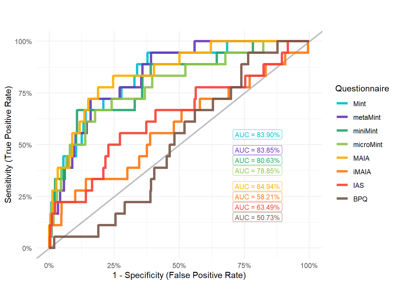
preds_addict <- compare_predictors("Disorders_Psychiatric_Addiction")
display_models(preds_addict$table, title="Best Predictor", subtitle = "Addiction")preds_addict$p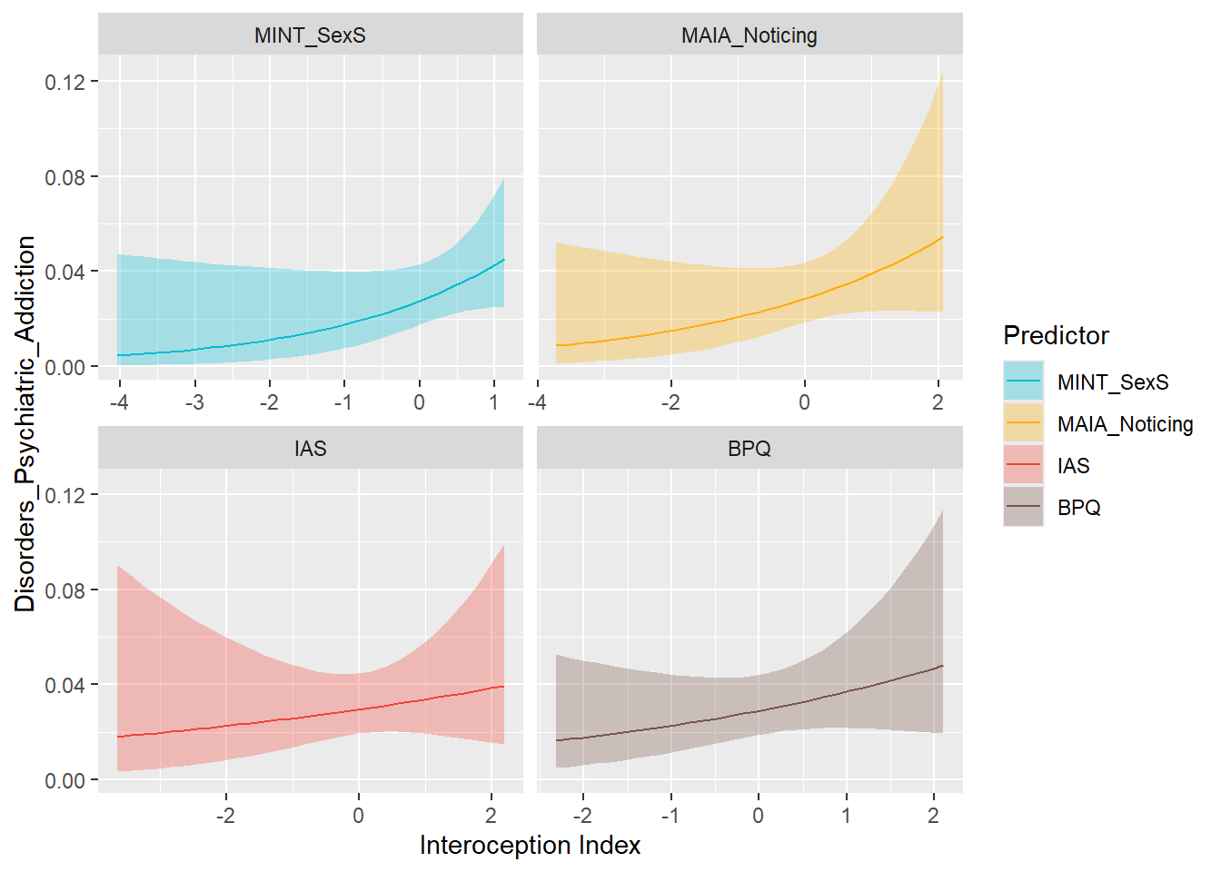
mods_addict <- compare_models_glm("Disorders_Psychiatric_Addiction")
display_models(mods_addict$table, title="Best Model", subtitle = "Addiction")mods_addict$p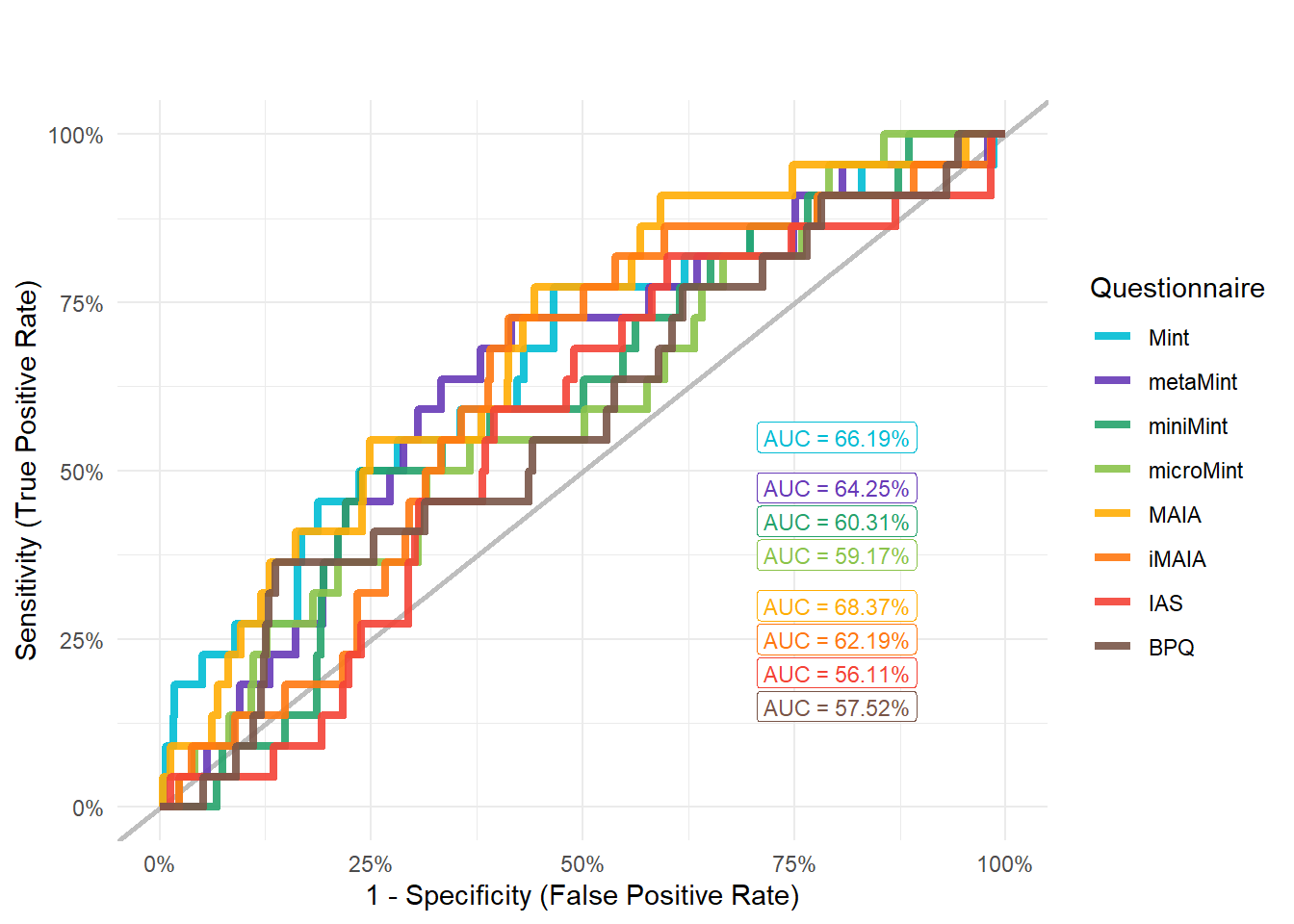
preds_adhd <- compare_predictors("Disorders_Psychiatric_ADHD")
display_models(preds_adhd$table, title="Best Predictor", subtitle = "ADHD")preds_adhd$p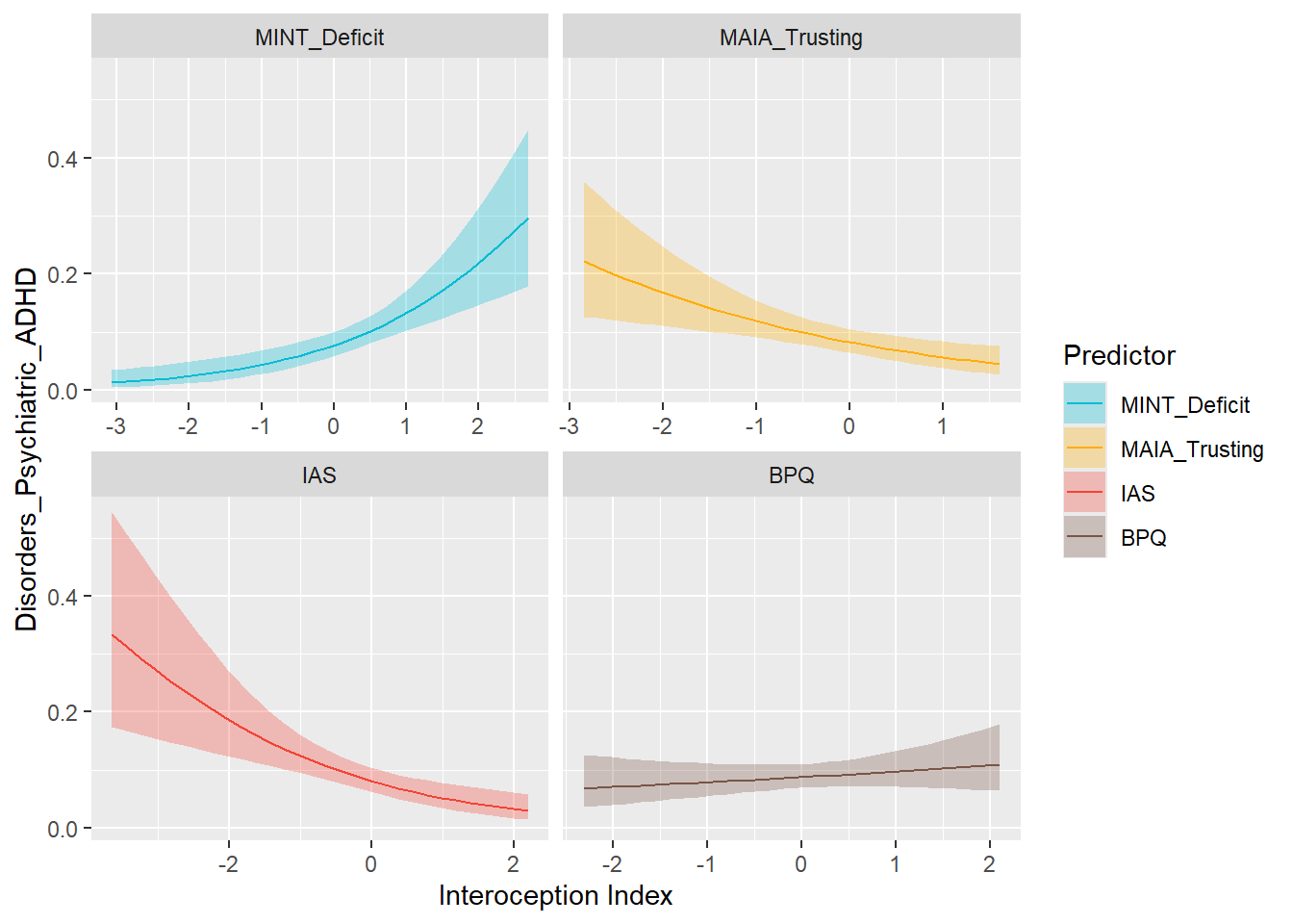
mods_adhd <- compare_models_glm("Disorders_Psychiatric_ADHD",
title = "ADHD", subtitle = "Attention Deficit/Hyperactivity Disorder")
display_models(mods_adhd$table, title="Best Model", subtitle = "ADHD")mods_adhd$p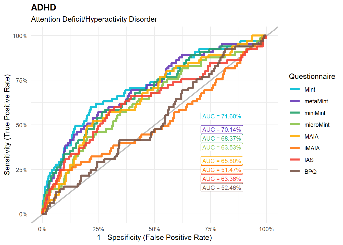
preds_asd <- compare_predictors("Disorders_Psychiatric_Autism")
display_models(preds_asd$table, title="Best Predictor", subtitle = "Autism")preds_asd$p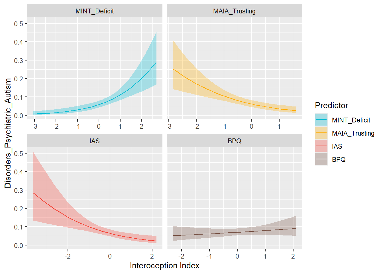
mods_asd <- compare_models_glm("Disorders_Psychiatric_Autism",
title = "ASD", subtitle = "Autism Spectrum Disorder")
display_models(mods_asd$table, title="Best Model", subtitle = "Autism")mods_asd$p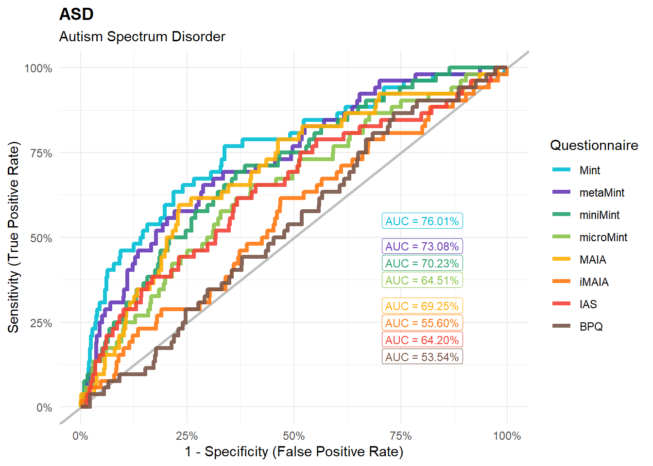
preds_bpd <- compare_predictors("Disorders_Psychiatric_Borderline")
display_models(preds_bpd$table, title="Best Predictor", subtitle = "Borderline Personality Disorder")preds_bpd$p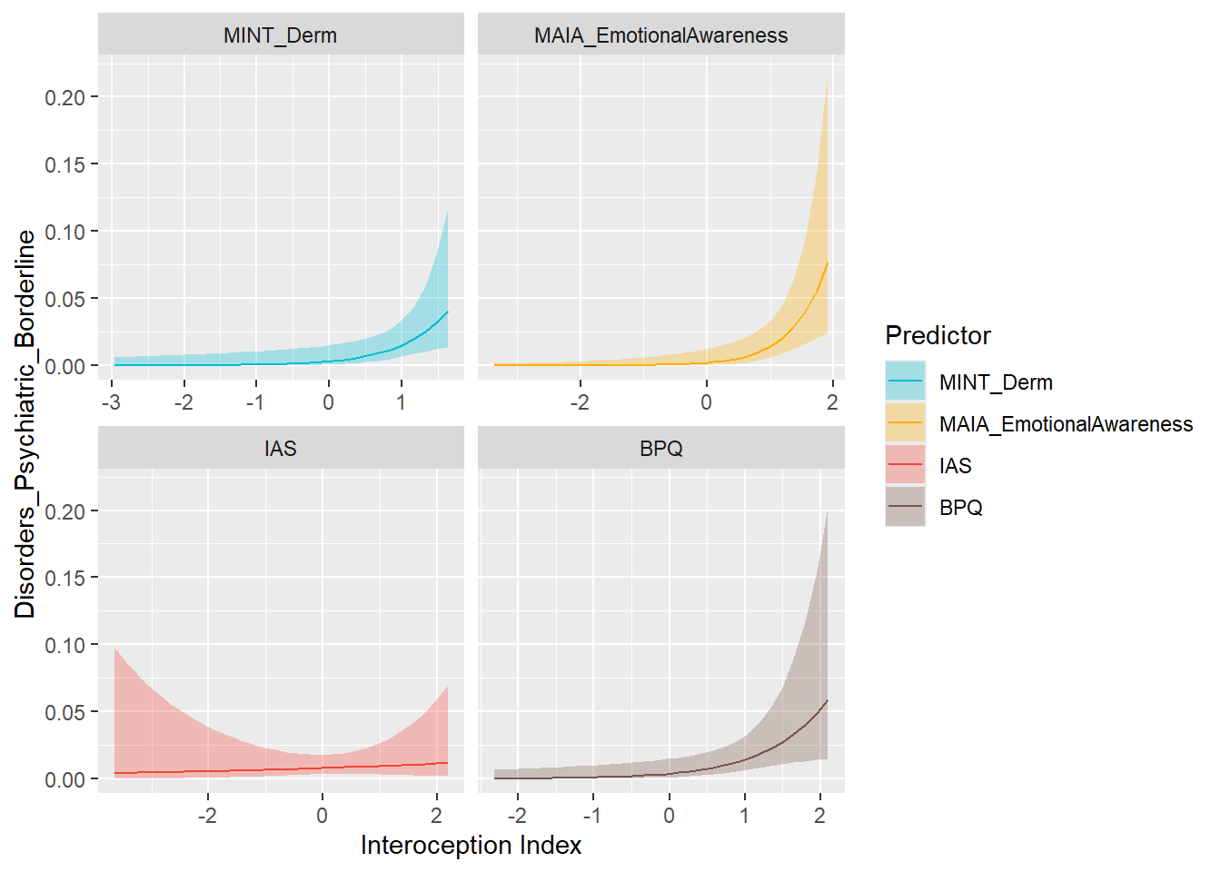
mods_bpd <- compare_models_glm("Disorders_Psychiatric_Borderline")
display_models(mods_bpd$table, title="Best Model", subtitle = "Borderline Personality Disorder")mods_bpd$p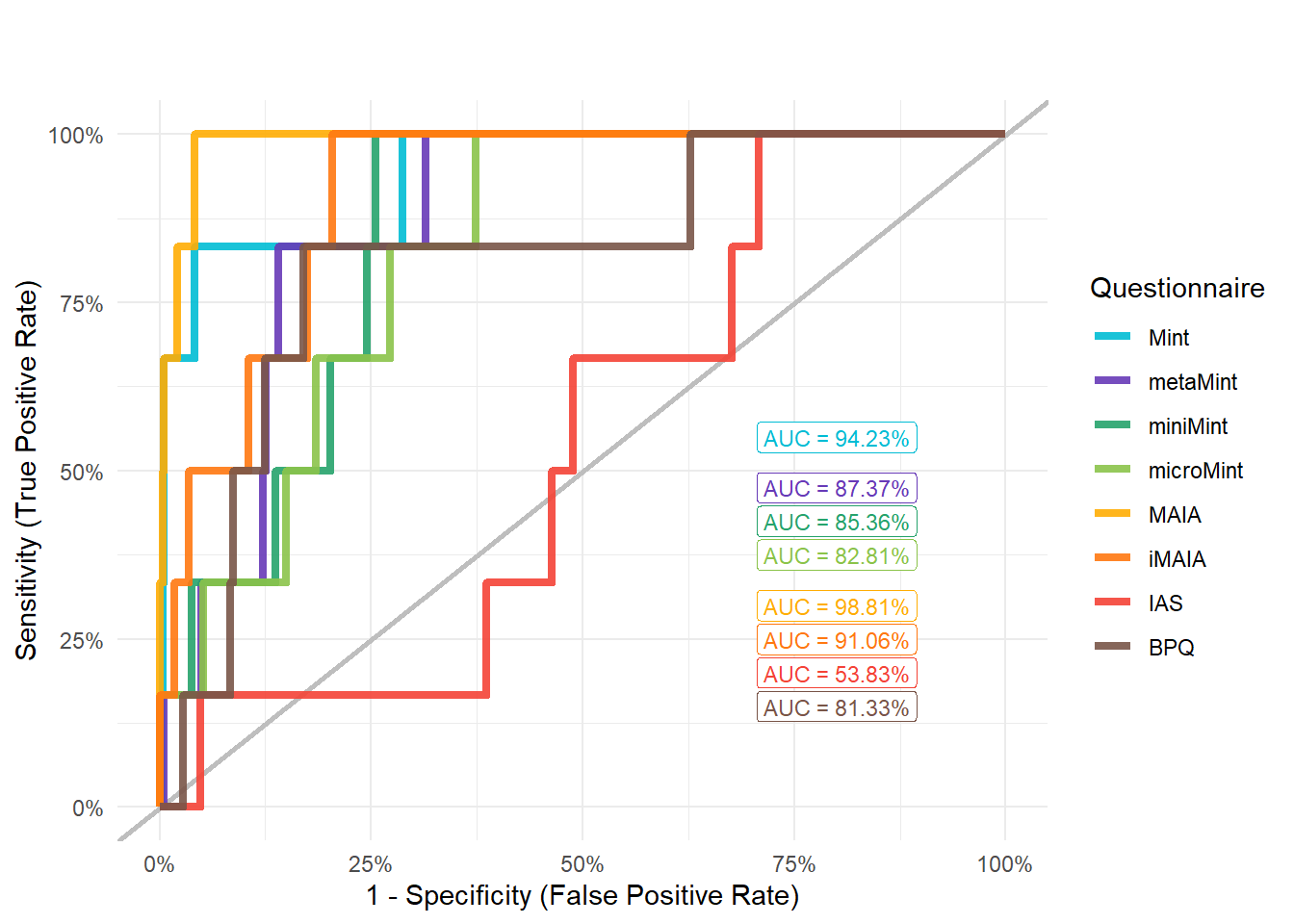
preds_afferent <- compare_predictors("Disorders_Somatic_AfferentSensitivity")
display_models(preds_afferent$table, title="Best Predictor", subtitle = "Afferent Sensitivity Symptoms")preds_afferent$p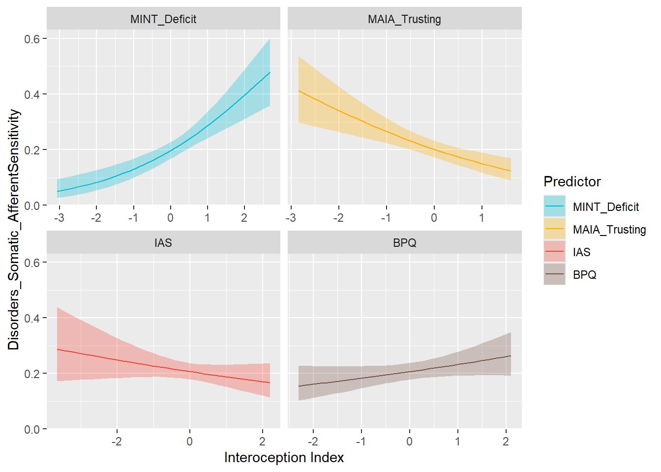
mods_afferent <- compare_models_glm("Disorders_Somatic_AfferentSensitivity",
title="Afferent Sensitivity Symptoms",
subtitle = "Migraine, neuropathy, muscle tension, dizziness, ...")
display_models(mods_afferent$table, title="Best Model", subtitle = "Afferent Sensitivity Symptoms")mods_afferent$p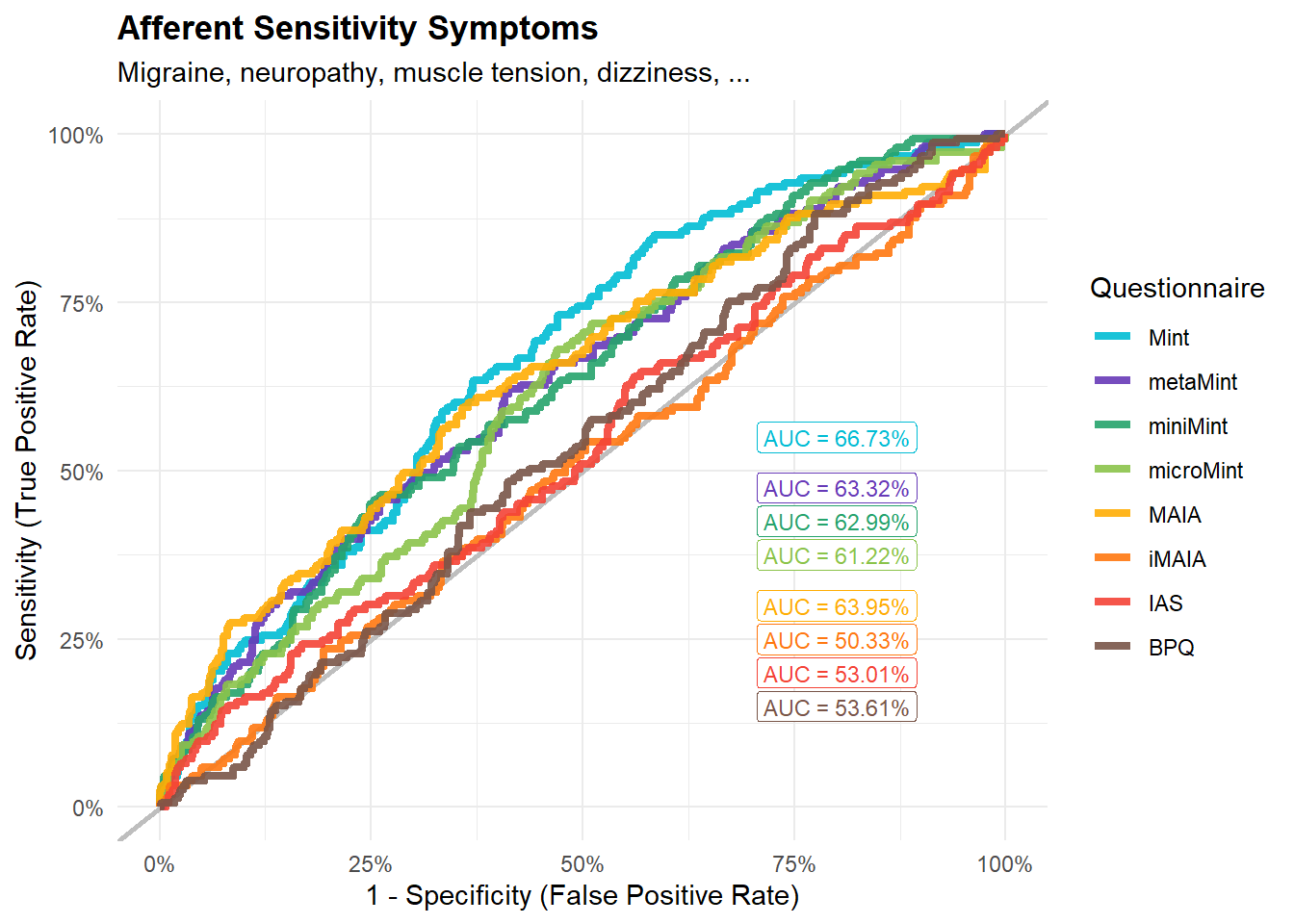
preds_central <- compare_predictors("Disorders_Somatic_CentralSensitization")
display_models(preds_central$table, title="Best Predictor", subtitle = "Central Sensitization Symptoms")preds_central$p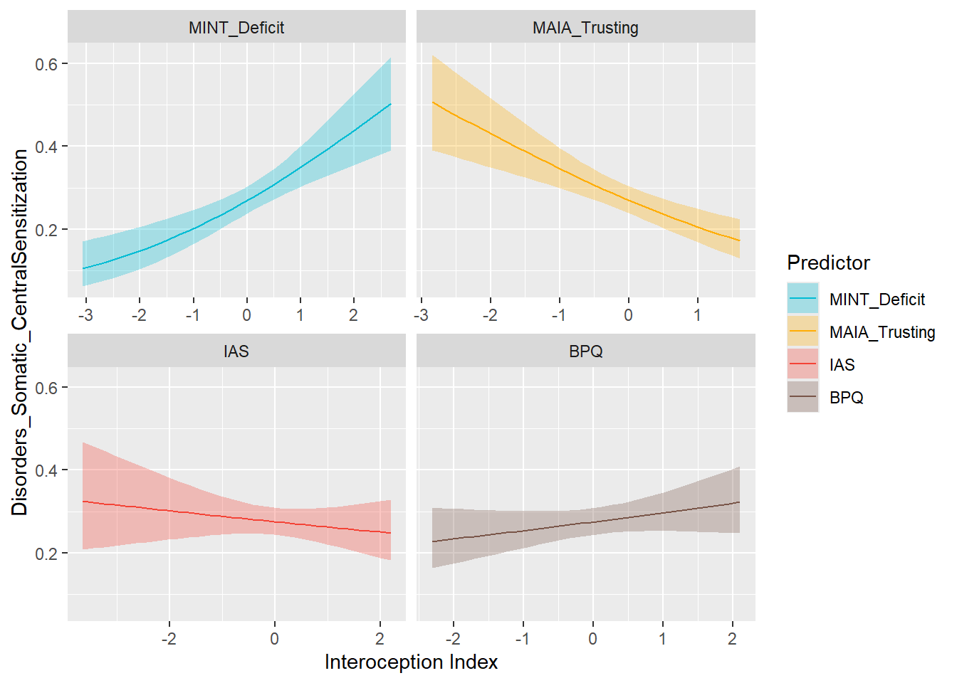
mods_central <- compare_models_glm("Disorders_Somatic_CentralSensitization",
title="Central Sensitization Symptoms",
subtitle = "Fibromyalgia, chronic fatigue, back pain, IBS, ...")
display_models(mods_central$table, title="Best Model", subtitle = "Central Sensitization Symptoms")mods_central$p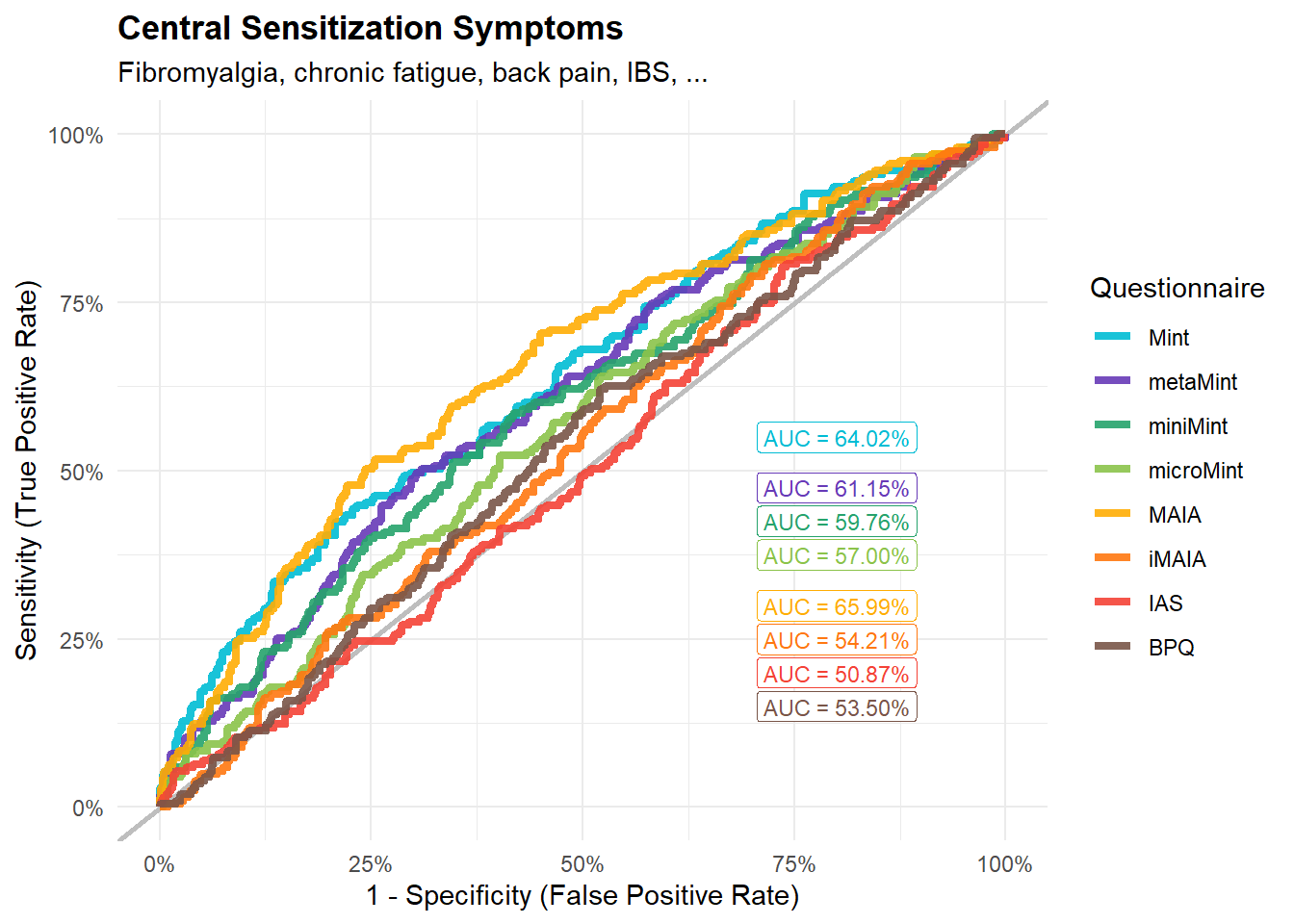
preds_autonomic <- compare_predictors("Disorders_Somatic_AutonomicDysfunction")
display_models(preds_autonomic$table, title="Best Predictor", subtitle = "Autonomic Dysfunction")preds_autonomic$p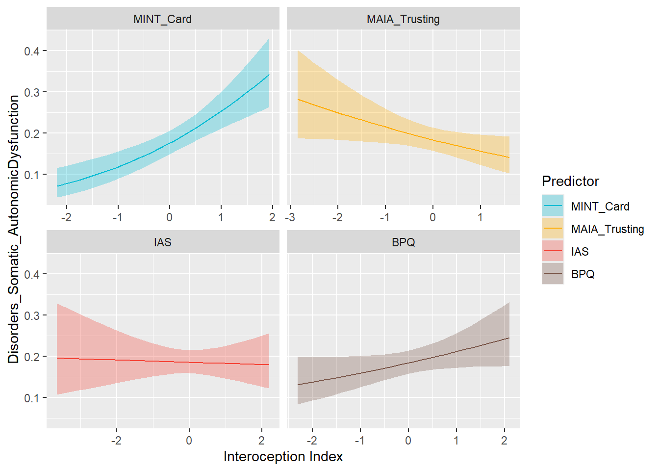
mods_autonomic <- compare_models_glm("Disorders_Somatic_AutonomicDysfunction",
title="Autonomic Dysfunction",
subtitle = "Hypermobility, chest pain, hypo/hypertension, ....")
display_models(mods_autonomic$table, title="Best Model", subtitle = "Autonomic Dysfunction")mods_autonomic$p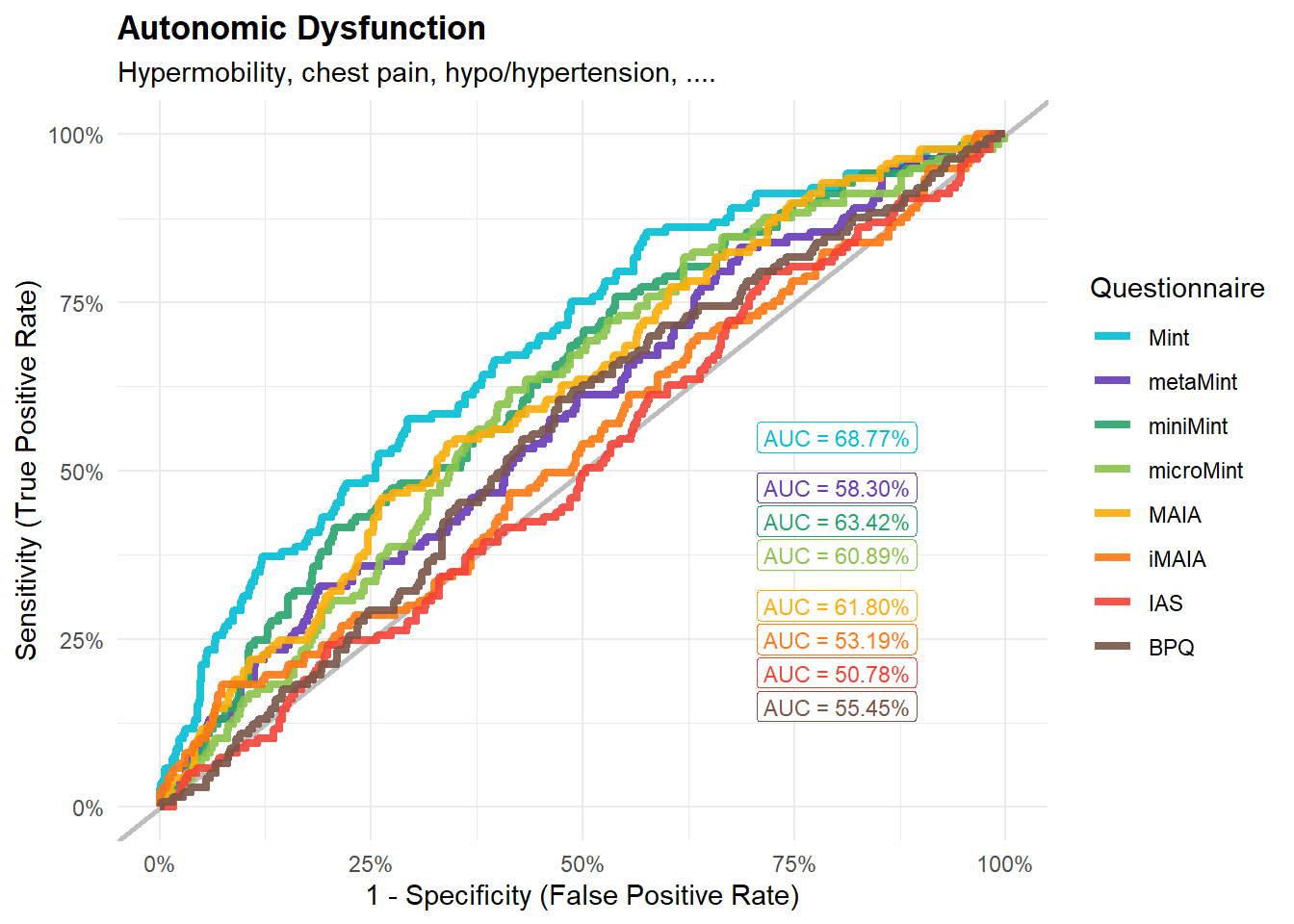
preds_immune <- compare_predictors("Disorders_Somatic_ImmuneInflammatory")
display_models(preds_immune$table, title="Best Predictor", subtitle = "Immune-Inflammatory Symptoms")preds_immune$p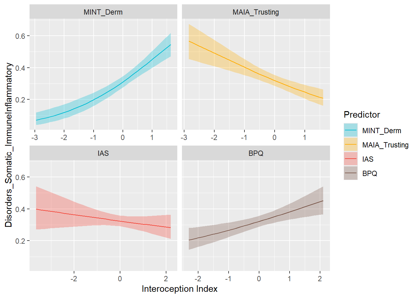
mods_immune <- compare_models_glm("Disorders_Somatic_ImmuneInflammatory",
title="Immune-Inflammatory Symptoms",
subtitle = "Allergies, asthma, eczema, autoimmune, ...")
display_models(mods_immune$table, title="Best Model", subtitle = "Immune-Inflammatory Symptoms")mods_immune$p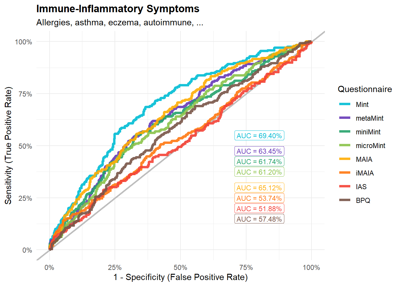
preds_age <- compare_predictors("Age")
display_models(preds_age$table, title="Best Predictor", subtitle = "Age")preds_age$p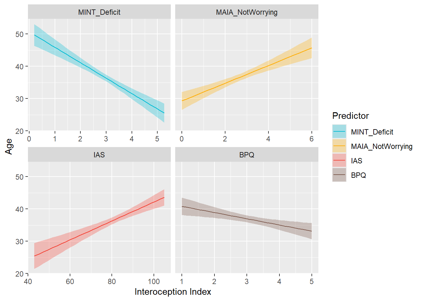
mods_age <- compare_models_lm("Age")
display_models(mods_age, title="Best Model", subtitle = "Age")df$Sex <- ifelse(df$Gender == "Female", 1, ifelse(df$Gender == "Male", 0, NA))
preds_sex <- compare_predictors("Sex")
display_models(preds_sex$table, title="Best Predictor", subtitle = "Sex")preds_sex$p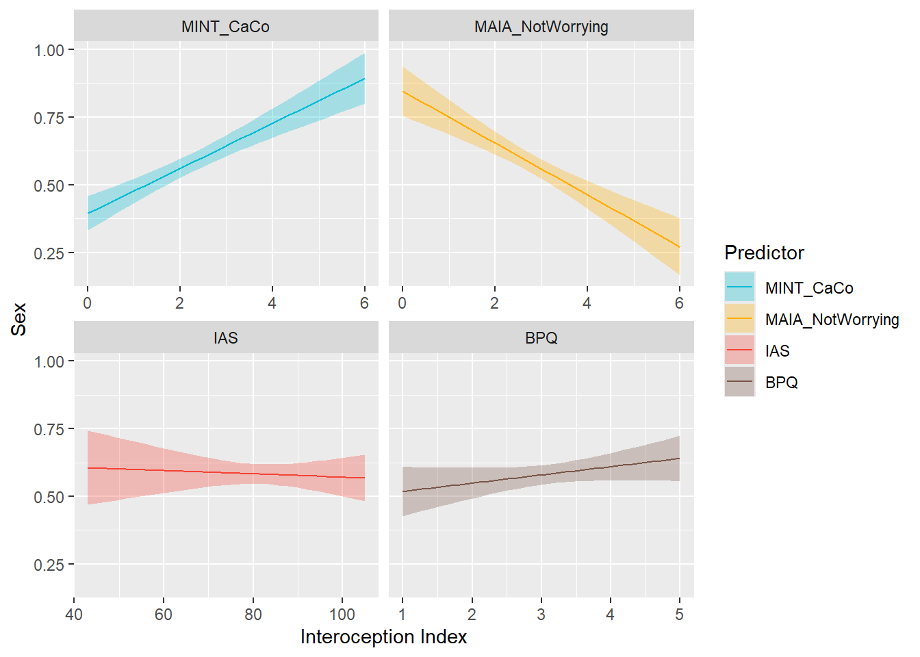
mods_sex <- compare_models_glm("Sex")
display_models(mods_sex$table, title="Best Model", subtitle = "Sex")mods_sex$p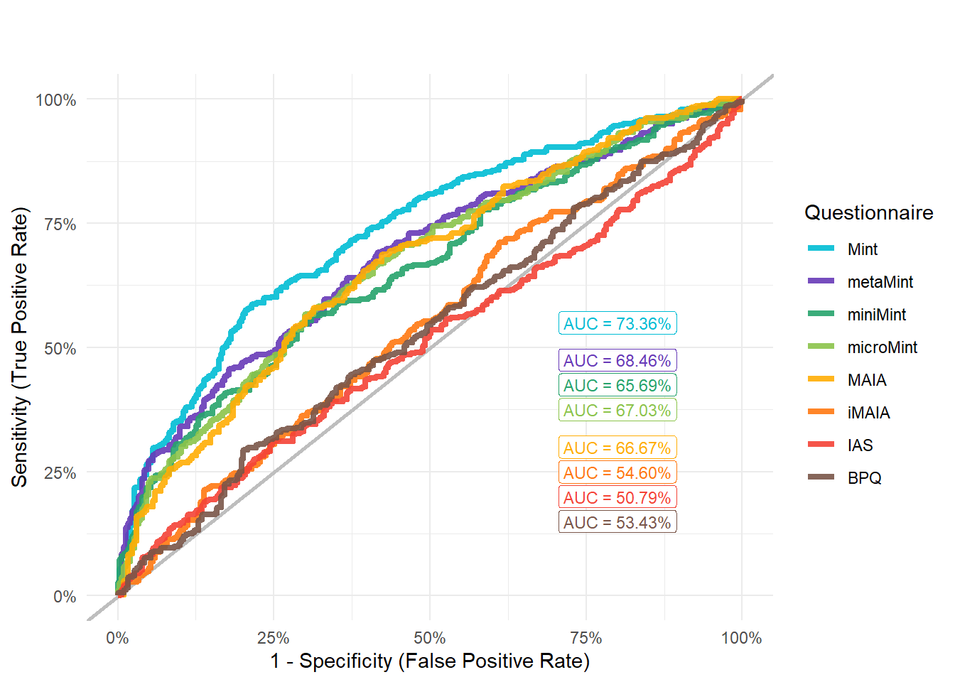
preds_bmi <- compare_predictors("BMI")
display_models(preds_bmi$table, title="Best Predictor", subtitle = "BMI")preds_bmi$p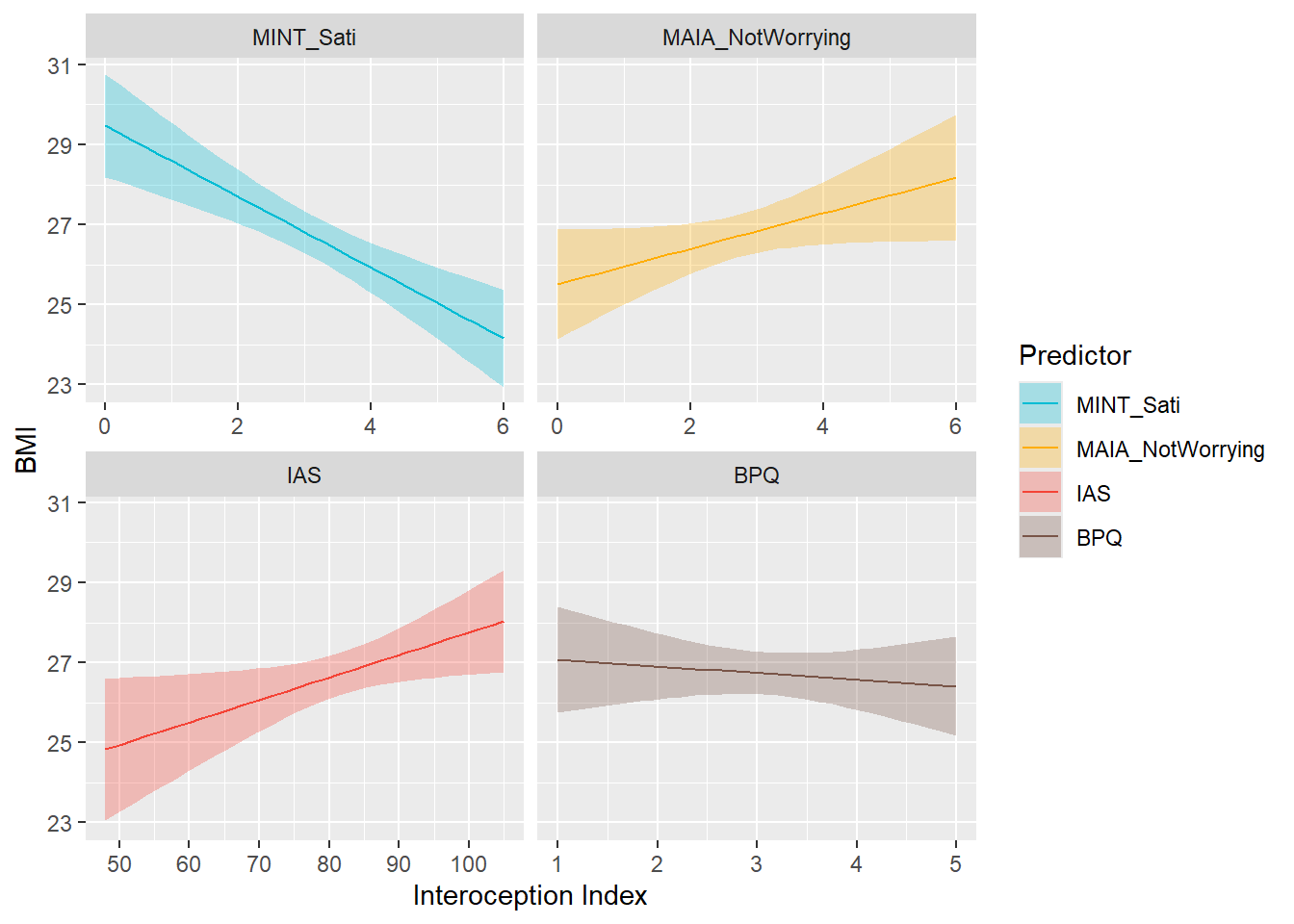
mods_bmi <- compare_models_lm("BMI")
display_models(mods_bmi, title="Best Model", subtitle = "BMI")preds_physactiv <- compare_predictors("Physical_Active")
display_models(preds_physactiv$table, title="Best Predictor", subtitle = "Physical Activity")preds_physactiv$p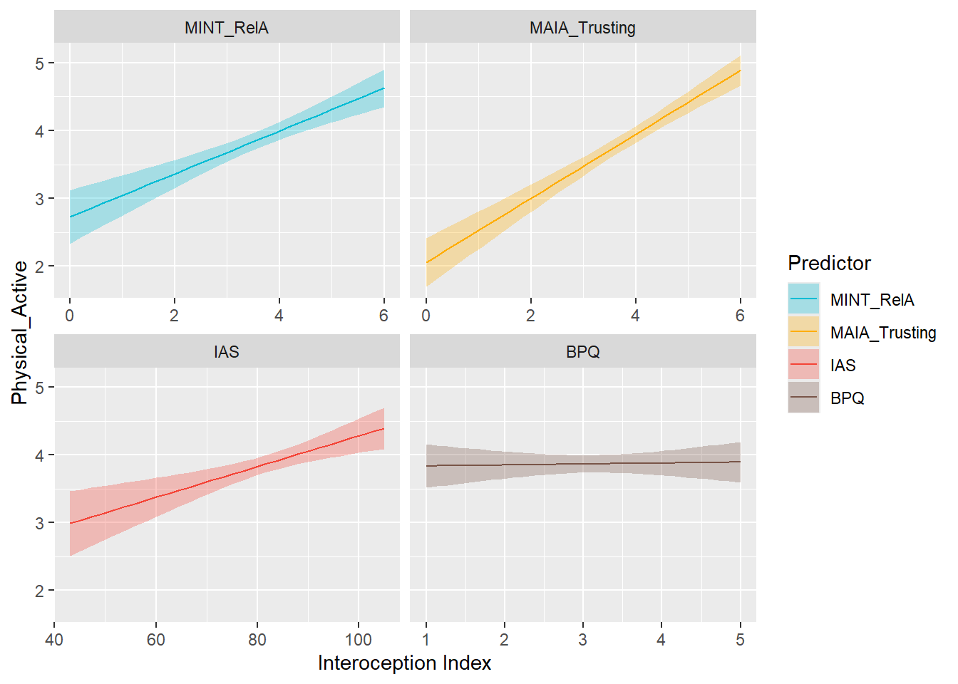
mods_physactiv <- compare_models_lm("Physical_Active")
display_models(mods_physactiv, title="Best Model", subtitle = "Physical Activity")preds_wearN <- compare_predictors("Wearables_Number", family = "poisson")
display_models(preds_wearN$table, title="Best Predictor", subtitle = "Wearables Number")preds_wearN$p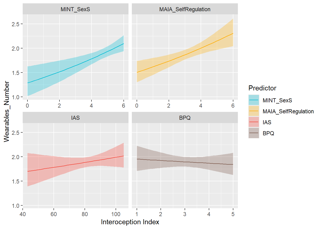
df$Wearables_HeartOwn <- ifelse(df$Wearables_Heart == "Not owning", 0, 1)
preds_wearHeartOwn <- compare_predictors("Wearables_HeartOwn")
display_models(preds_wearHeartOwn$table, title="Best Predictor", subtitle = "Wearables Heart Ownership")preds_wearHeartOwn$p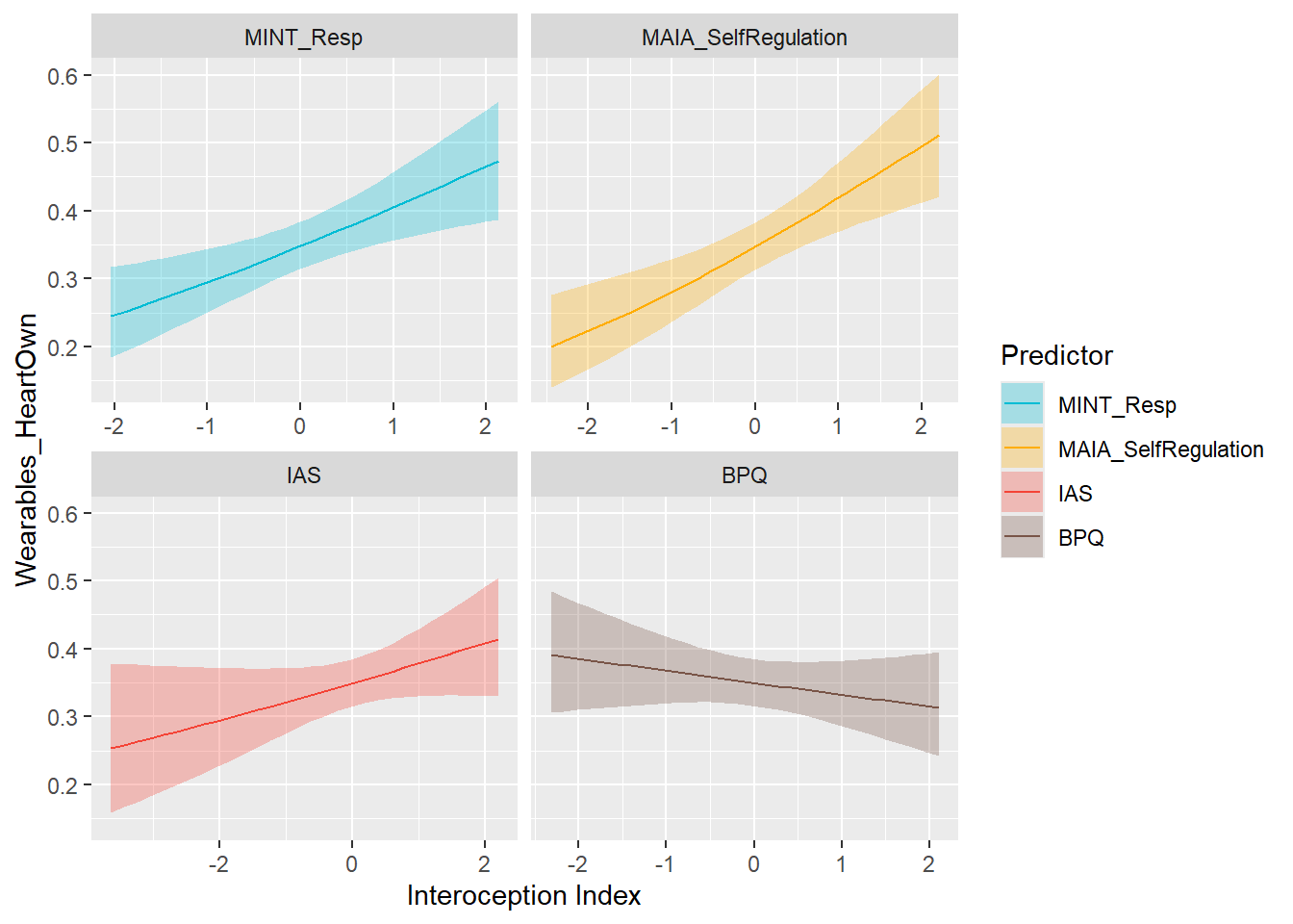
mods_wearHeartOwn <- compare_models_glm("Wearables_HeartOwn")
display_models(mods_wearHeartOwn$table, title="Best Model", subtitle = "Wearables Heart Ownership")mods_wearHeartOwn$p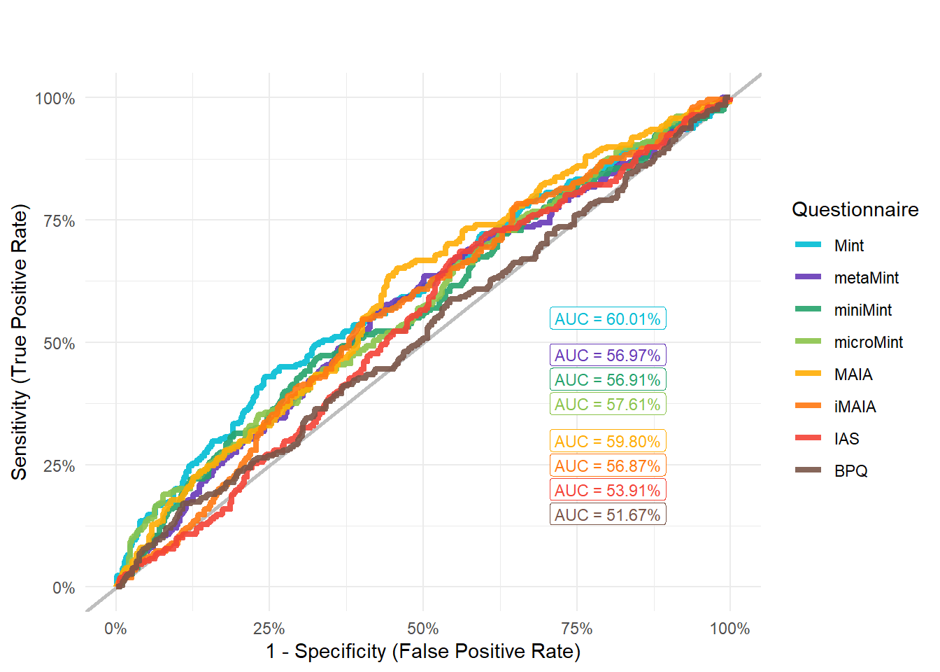
preds_wearHeartImp <- compare_predictors("Wearables_HeartImportance")
display_models(preds_wearHeartImp$table, title="Best Predictor", subtitle = "Wearables Heart Importance")preds_wearHeartImp$p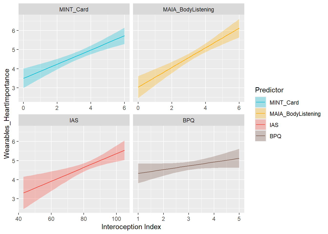
mods_wearHeartImp <- compare_models_lm("Wearables_HeartImportance")
display_models(mods_wearHeartImp, title="Best Model", subtitle = "Wearables Heart Importance")df$Wearables_SleepOwn <- ifelse(df$Wearables_Sleep == "Not owning", 0, 1)
preds_wearSleepOwn <- compare_predictors("Wearables_SleepOwn")
display_models(preds_wearSleepOwn$table, title="Best Predictor", subtitle = "Wearables Sleep Ownership")preds_wearSleepOwn$p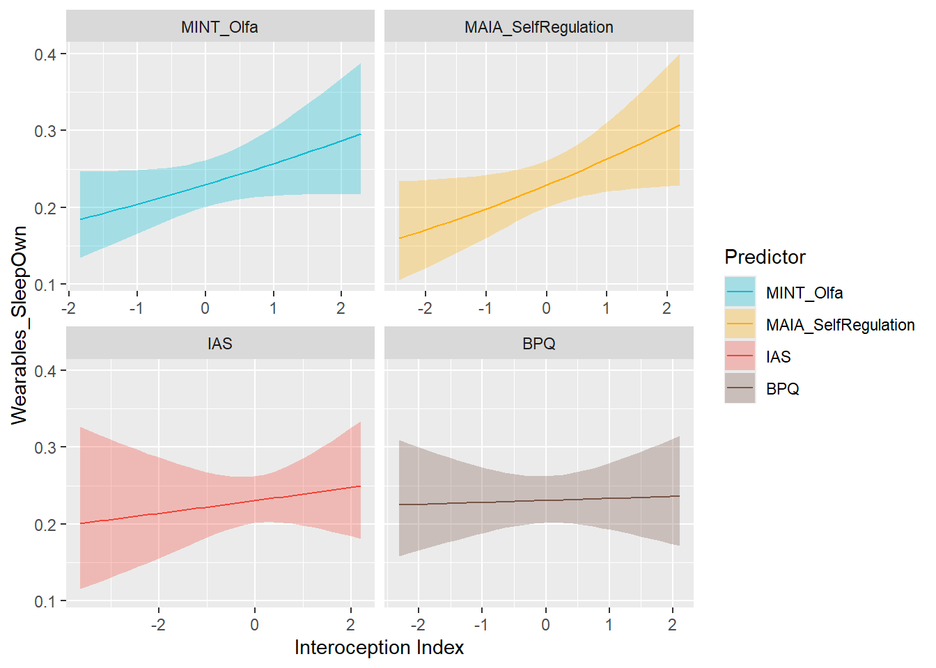
mods_wearSleepOwn <- compare_models_glm("Wearables_SleepOwn")
display_models(mods_wearSleepOwn$table, title="Best Model", subtitle = "Wearables Sleep Ownership")preds_wearSleepImp <- compare_predictors("Wearables_SleepImportance")
display_models(preds_wearSleepImp$table, title="Best Predictor", subtitle = "Wearables Sleep Importance")preds_wearSleepImp$p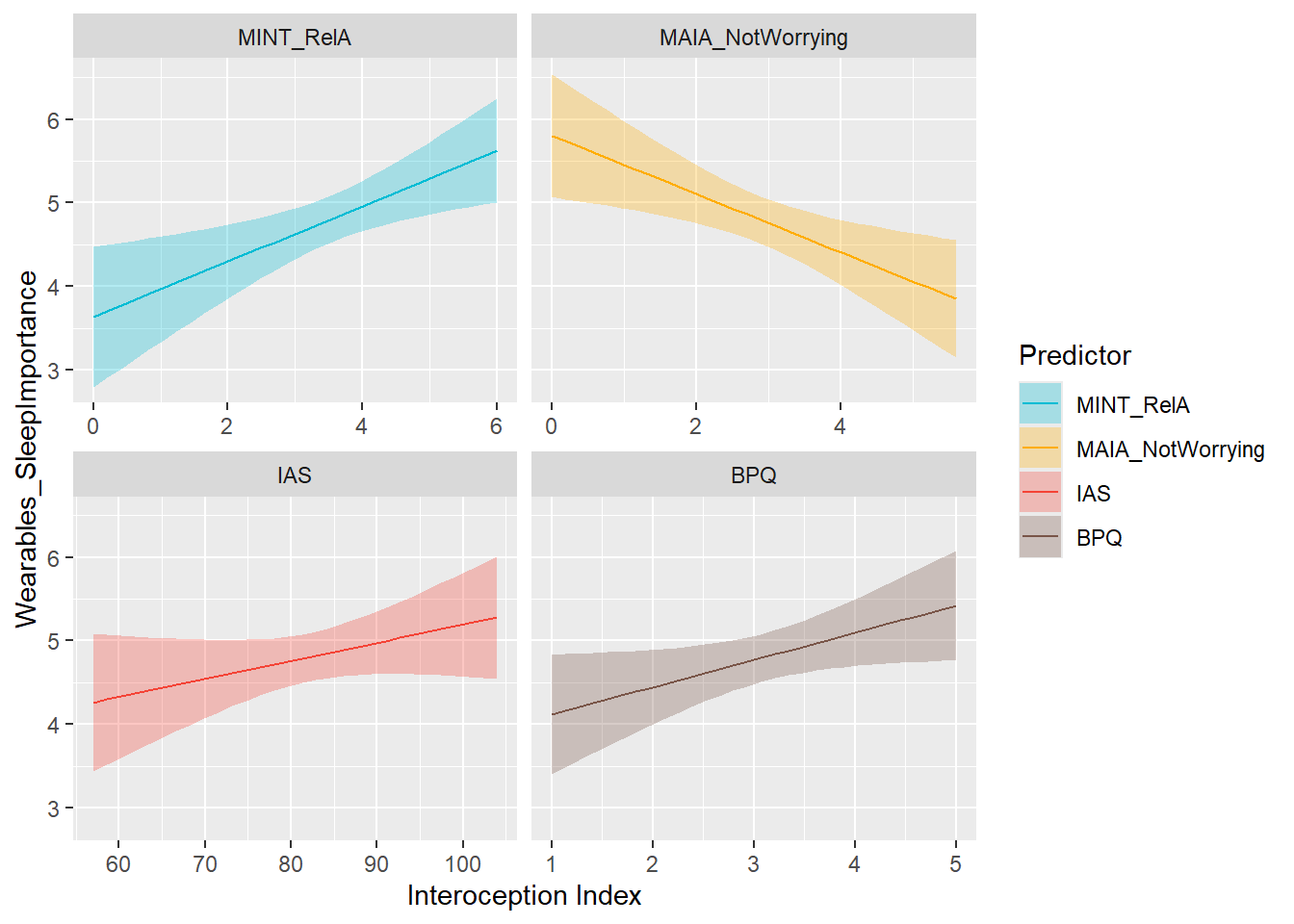
mods_wearSleepImp <- compare_models_lm("Wearables_SleepImportance")
display_models(mods_wearSleepImp, title="Best Model", subtitle = "Wearables Sleep Importance")df$Wearables_StepsOwn <- ifelse(df$Wearables_Steps == "Not owning", 0, 1)
preds_wearStepsOwn <- compare_predictors("Wearables_StepsOwn")
display_models(preds_wearStepsOwn$table, title="Best Predictor", subtitle = "Wearables Steps Ownership")preds_wearStepsOwn$p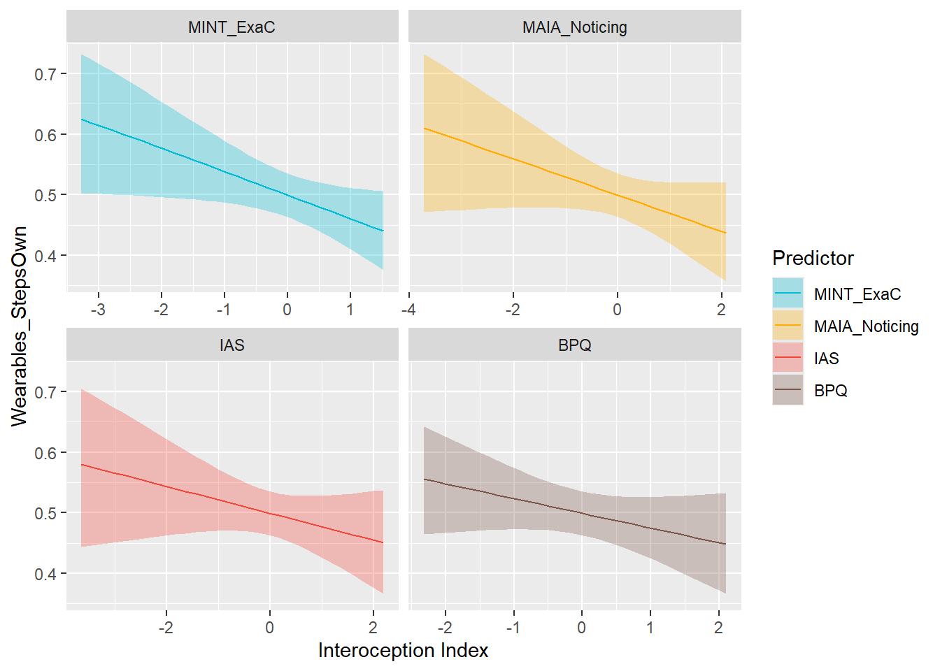
mods_wearStepsOwn <- compare_models_glm("Wearables_StepsOwn")
display_models(mods_wearStepsOwn$table, title="Best Model", subtitle = "Wearables Steps Ownership")preds_wearStepsImp <- compare_predictors("Wearables_StepsImportance")
display_models(preds_wearStepsImp$table, title="Best Predictor", subtitle = "Wearables Steps Importance")preds_wearStepsImp$p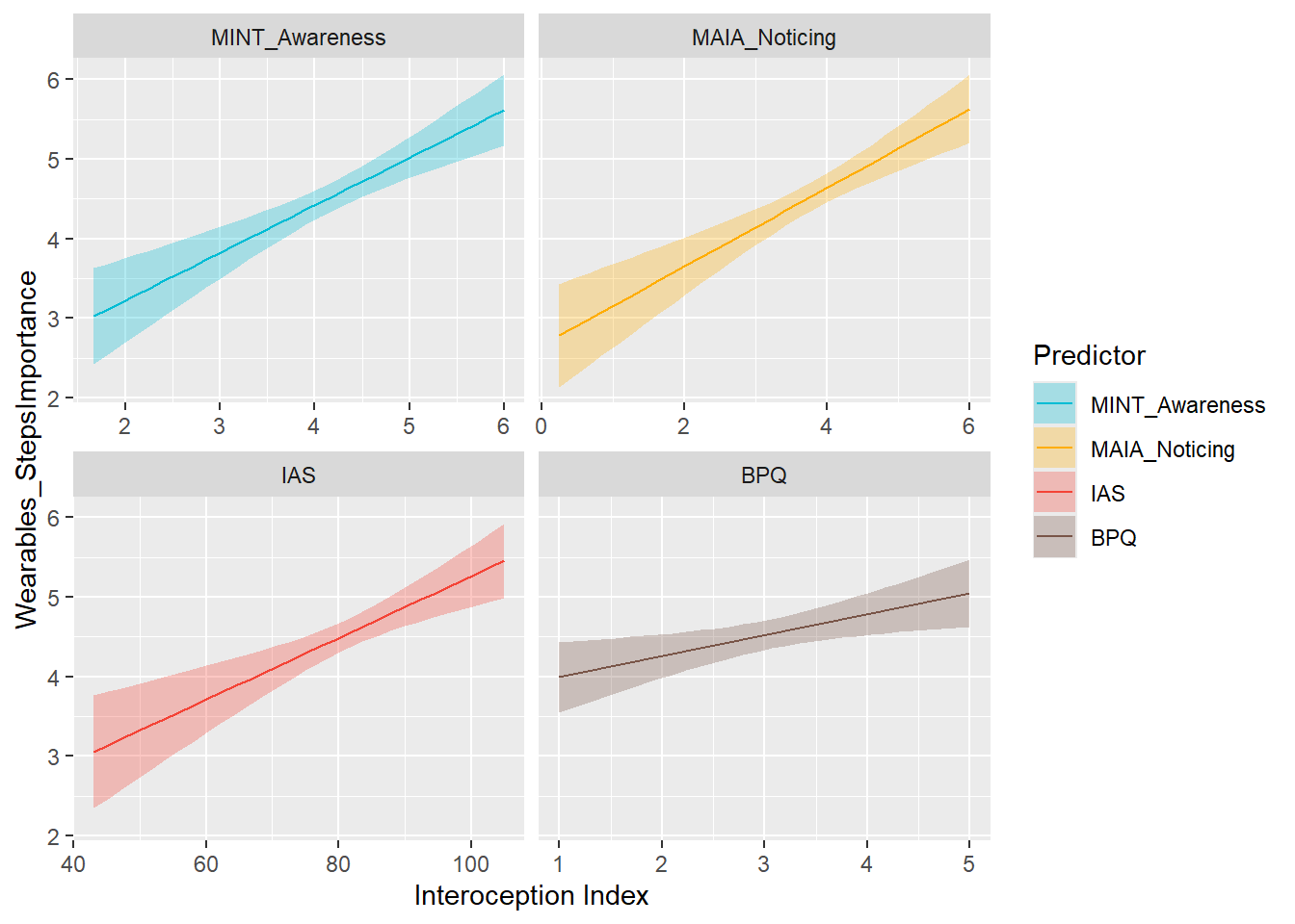
mods_wearStepsImp <- compare_models_lm("Wearables_StepsImportance")
display_models(mods_wearStepsImp, title="Best Model", subtitle = "Wearables Steps Importance")df$Wearables_WeightOwn <- ifelse(df$Wearables_Weight == "Not owning", 0, 1)
preds_wearWeightOwn <- compare_predictors("Wearables_WeightOwn")
display_models(preds_wearWeightOwn$table, title="Best Predictor", subtitle = "Wearables Weight Ownership")preds_wearWeightOwn$p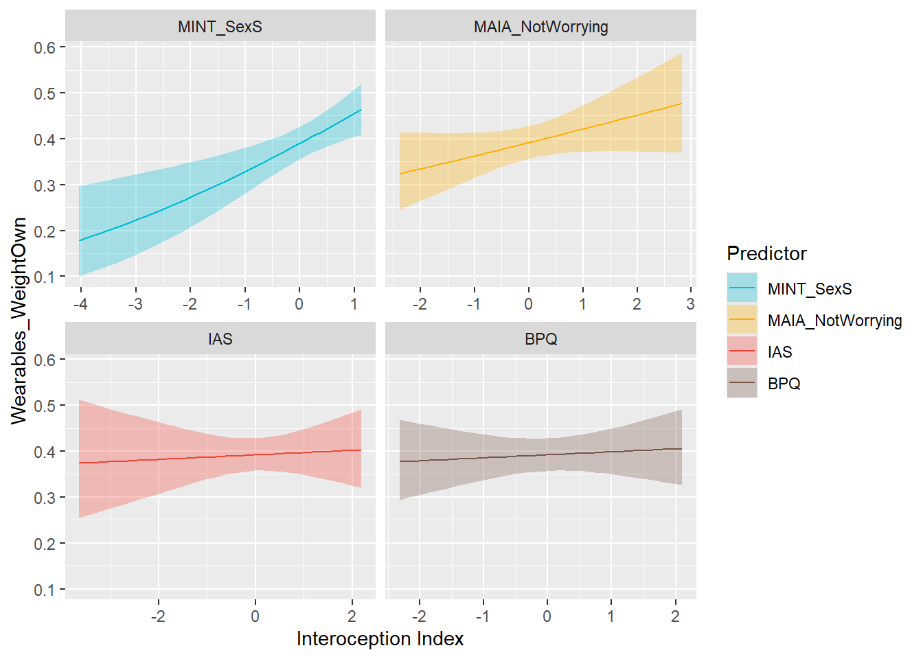
mods_wearWeightOwn <- compare_models_glm("Wearables_WeightOwn")
display_models(mods_wearWeightOwn$table, title="Best Model", subtitle = "Wearables Weight Ownership")preds_wearWeightImp <- compare_predictors("Wearables_WeightImportance")
display_models(preds_wearWeightImp$table, title="Best Predictor", subtitle = "Wearables Weight Importance")preds_wearWeightImp$p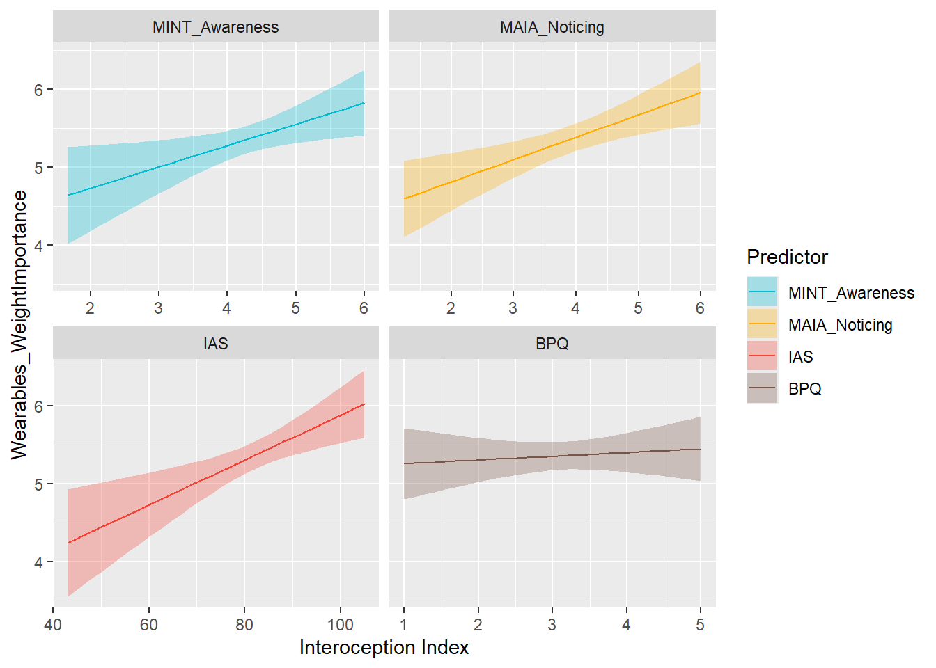
mods_wearWeightImp <- compare_models_lm("Wearables_WeightImportance")
display_models(mods_wearWeightImp, title="Best Model", subtitle = "Wearables Weight Importance")make_table1 <- function(preds=preds_dif, mods=mods_dif, group = "Alexithymia", outcome = "TAS - DIF") {
yvar <- preds$outcome
preds <- preds$table
best_pred_mint <- preds[str_detect(preds$Name, "MINT"), ]
best_pred_nonmint <- preds[!str_detect(preds$Name, "MINT"), ]
best_pred_nonmint <- best_pred_nonmint[best_pred_nonmint$R2 == max(best_pred_nonmint$R2), ][1,]
best_models_R2 <- str_remove(arrange(mods, desc(as.numeric(R2)))$Name, "m_")
best_model_BIC <- str_remove(arrange(mods, as.numeric(BIC))$Name, "m_")
if(length(unique(df[[yvar]])) > 2) {
# LMs - display correlation
r_mint <- cor.test(cbind(df, metamint)[[best_pred_mint$Name[1]]], df[[yvar]])
r_mint <- paste0(insight::format_value(r_mint$estimate, zap_small = TRUE))
r_nonmint <- cor.test(df[[best_pred_nonmint$Name[1]]], df[[yvar]])
r_nonmint <- paste0(insight::format_value(r_nonmint$estimate, zap_small = TRUE))
} else {
# GLMs - display log-odds
r_mint <- insight::format_value(best_pred_mint$Coefficient)
r_nonmint <- insight::format_value(best_pred_nonmint$Coefficient)
}
# Format
best_models_R2[str_detect(best_models_R2, "mint")] <- paste0("<b>", best_models_R2[str_detect(best_models_R2, "mint")], "</b>")
best_model_BIC[str_detect(best_model_BIC, "mint")] <- paste0("<b>", best_model_BIC[str_detect(best_model_BIC, "mint")], "</b>")
best_models_R2 <- paste0("<small>", paste0(best_models_R2, collapse = " > "), "</small>")
best_model_BIC <- paste0("<small>", paste0(best_model_BIC, collapse = " > "), "</small>")
data.frame(
Group = group,
Outcome = outcome,
Best_MINT_Predictor = paste0(str_remove(best_pred_mint$Name[1], "MINT_"), "<br><small><i>(", r_mint, ")</i></small>"),
Best_NonMINT_Predictor = paste0(str_replace(best_pred_nonmint$Name[1], "_", " - "), "<br><small><i>(", r_nonmint, ")</i></small>"),
Best_Models_R2 = best_models_R2,
Best_Models_BIC = best_model_BIC
)
}
rez <- rbind(
make_table1(preds_dif, mods_dif, group = "Alexithymia", outcome = "Difficulty Identifying Feelings (DIF)<small><p align='right'><i>TAS-20</i></small><p>"),
make_table1(preds_ddf, mods_ddf, group = "Alexithymia", outcome = "Difficulty Describing Feelings (DDF)<small><p align='right'><i>TAS-20</i></small><p>"),
make_table1(preds_eot, mods_eot, group = "Alexithymia", outcome = "Externally Oriented Thinking (EOT)<small><p align='right'><i>TAS-20</i></small><p>"),
make_table1(preds_arou, mods_arou, group = "Emotion Reactivity", outcome = "Arousal<small><p align='right'><i>ERS</i></small><p>"),
make_table1(preds_sens, mods_sens, group = "Emotion Reactivity", outcome = "Sensitivity<small><p align='right'><i>ERS</i></small><p>"),
make_table1(preds_pers, mods_pers, group = "Emotion Reactivity", outcome = "Persistence<small><p align='right'><i>ERS</i></small><p>"),
make_table1(preds_ls, mods_ls, group = "Mood", outcome = "Life Satisfaction"),
make_table1(preds_anx, mods_anx, group = "Mood", outcome = "Anxiety<small><p align='right'><i>PHQ-4</i></small><p>"),
make_table1(preds_dep, mods_dep, group = "Mood", outcome = "Depression<small><p align='right'><i>PHQ-4</i></small><p>"),
make_table1(preds_moodt, mods_moodt$table, group = "Mental Health", outcome = "Mood Disorder"),
make_table1(preds_adhd, mods_adhd$table, group = "Mental Health", outcome = "ADHD"),
make_table1(preds_asd, mods_asd$table, group = "Mental Health", outcome = "Autism"),
make_table1(preds_afferent, mods_afferent$table, group = "Somatic Health", outcome = "Afferent Sensitivity<small><small><p align='right'><i>Migraine, neuropathy, muscle tension, dizziness, ...</i></small></small><p>"),
make_table1(preds_central, mods_central$table, group = "Somatic Health", outcome = "Central Sensitization<small><small><p align='right'><i>Fibromyalgia, chronic fatigue, back pain, IBS, ...</i></small></small><p>"),
make_table1(preds_autonomic, mods_autonomic$table, group = "Somatic Health", outcome = "Autonomic Dysfunction<small><small><p align='right'><i>Hypermobility, chest pain, hypo/hypertension, ...</i></small></small><p>"),
make_table1(preds_immune, mods_immune$table, group = "Somatic Health", outcome = "Immune-Inflammatory<small><small><p align='right'><i>Allergies, eczema, autoimmune, ...</i></small></small><p>"),
make_table1(preds_cefsabody, mods_cefsabody, group = "Dissociative Symptoms", outcome = "Body<small><p align='right'><i>CEFSA</i></small><p>"),
make_table1(preds_cefsaself, mods_cefsaself, group = "Dissociative Symptoms", outcome = "Self<small><p align='right'><i>CEFSA</i></small><p>"),
make_table1(preds_cefsaemo, mods_cefsaemo, group = "Dissociative Symptoms", outcome = "Emotions<small><p align='right'><i>CEFSA</i></small><p>"),
make_table1(preds_cefsareal, mods_cefsareal, group = "Dissociative Symptoms", outcome = "Reality<small><p align='right'><i>CEFSA</i></small><p>"),
# make_table1(preds_pialive, mods_pialive, group = "Primals", outcome = "Alive<small><p align='right'><i>PI-18</i></small><p>"),
# make_table1(preds_pisafe, mods_pisafe, group = "Primals", outcome = "Safe<small><p align='right'><i>PI-18</i></small><p>"),
# make_table1(preds_pient, mods_pient, group = "Primals", outcome = "Enticing<small><p align='right'><i>PI-18</i></small><p>"),
# make_table1(preds_pigood, mods_pigood, group = "Primals", outcome = "Good<small><p align='right'><i>PI-18</i></small><p>")
make_table1(preds_bmi, mods_bmi, group = "Lifestyle", outcome = "BMI"),
make_table1(preds_physactiv, mods_physactiv, group = "Lifestyle", outcome = "Physical Activity"),
# make_table1(preds_age, mods_age, group = "Lifestyle", outcome = "Age"),
make_table1(preds_wearHeartImp, mods_wearHeartImp, group = "Lifestyle", outcome = "Cardiac Monitoring"),
make_table1(preds_wearSleepImp, mods_wearSleepImp, group = "Lifestyle", outcome = "Sleep Monitoring"),
make_table1(preds_wearStepsImp, mods_wearStepsImp, group = "Lifestyle", outcome = "Steps Monitoring")
# make_table1(preds_wearWeightImp, mods_wearWeightImp, group = "Lifestyle", outcome = "Weight Monitoring")
)
tab2 <- rez |>
gt::gt() |>
gt::tab_header(
title = gt::md("**Interoception Questionnaires Comparison**"),
subtitle = "MINT vs. MAIA, IAS, BPQ"
) |>
gt::cols_width(
Outcome ~ gt::pct(23),
Best_MINT_Predictor ~ gt::pct(12),
Best_NonMINT_Predictor ~ gt::pct(15),
Best_Models_R2 ~ gt::pct(25),
Best_Models_BIC ~ gt::pct(25)
) |>
gt::tab_style(
style = gt::cell_text(weight="bold", v_align = "middle"),
locations = gt::cells_column_labels()
) |>
gt::tab_style(
style = gt::cell_text(align = "center", v_align = "middle"),
locations = gt::cells_body(columns=c("Best_MINT_Predictor", "Best_NonMINT_Predictor"))
) |>
gt::tab_row_group(
label = "Lifestyle",
rows = Group == "Lifestyle"
) |>
gt::tab_row_group(
label = "Dissociative Symptoms",
rows = Group == "Dissociative Symptoms"
) |>
gt::tab_row_group(
label = "Primal World Beliefs",
rows = Group == "Primals"
) |>
gt::tab_row_group(
label = "Somatic Health",
rows = Group == "Somatic Health"
) |>
gt::tab_row_group(
label = "Mental Health",
rows = Group == "Mental Health"
) |>
gt::tab_row_group(
label = "Mood",
rows = Group == "Mood"
) |>
gt::tab_row_group(
label = "Emotional Reactivity",
rows = Group == "Emotion Reactivity"
) |>
gt::tab_row_group(
label = "Alexithymia",
rows = Group == "Alexithymia"
) |>
gt::tab_style(
style = list(
gt::cell_fill(color = "gray85"),
gt::cell_text(weight="bold", style="italic")),
locations = gt::cells_row_groups()
) |>
gt::tab_style(
style = gt::cell_fill(color = "#81C784"),
locations = list(
gt::cells_body(columns="Best_MINT_Predictor", rows=c(1:4, 11:18, 20:21, 24))
)
) |>
gt::tab_style(
style = gt::cell_fill(color = "#FFB74D"),
locations = list(
gt::cells_body(columns="Best_MINT_Predictor", rows=c(5:9, 10, 19, 22))
)
) |>
gt::tab_style(
style = gt::cell_fill(color = "#EF9A9A"),
locations = list(
gt::cells_body(columns="Best_MINT_Predictor", rows=c(23, 25))
)
) |>
gt::tab_style(
style = gt::cell_fill(color = "#81C784"),
locations = list(
gt::cells_body(columns="Best_Models_R2", rows=c(1:3, 11:13, 15:21, 23:25))
)
) |>
gt::tab_style(
style = gt::cell_fill(color = "#FFB74D"),
locations = list(
gt::cells_body(columns="Best_Models_R2", rows=c(4:10, 14, 22))
)
) |>
gt::tab_style(
style = gt::cell_fill(color = "#81C784"),
locations = list(
gt::cells_body(columns="Best_Models_BIC", rows=c(1:3, 11:20, 25))
)
) |>
gt::tab_style(
style = gt::cell_fill(color = "#FFB74D"),
locations = list(
gt::cells_body(columns="Best_Models_BIC", rows=c(4:10, 22))
)
) |>
gt::tab_style(
style = gt::cell_fill(color = "#EF9A9A"),
locations = list(
gt::cells_body(columns="Best_Models_BIC", rows=c(21, 23, 24))
)
) |>
gt::cols_label(
Best_MINT_Predictor = "Best Predictor\n(MINT)",
Best_NonMINT_Predictor = "Best Predictor\n(Non-MINT)",
Best_Models_R2 = "Best Models (R2)",
Best_Models_BIC = "Best Models (BIC)"
) |>
gt::cols_hide(Group) |>
gt::fmt_markdown() |>
gt::tab_options(
table.font.size = gt::pct(125)
)
tab2 |>
gt::tab_options(
table.font.size = gt::pct(50)
) |>
gt::opt_interactive()# gt::gtsave(tab2, "figures/table2.png", vwidth=1400, expand=0, quiet=TRUE)
# gt::gtsave(tab2, "figures/table2b.png", vwidth=1600, expand=0, quiet=TRUE)
tab2 |>
gt::cols_width(
Outcome ~ gt::pct(21),
Best_MINT_Predictor ~ gt::pct(17),
Best_NonMINT_Predictor ~ gt::pct(18),
Best_Models_R2 ~ gt::pct(22),
Best_Models_BIC ~ gt::pct(22)
) |>
gt::gtsave("figures/table2.png", vwidth=1700, expand=0, quiet=TRUE)fig1a <- patchwork::wrap_elements(
patchwork::wrap_elements(grid::rasterGrob(png::readPNG("figures/fig1a.png"))) +
patchwork::plot_annotation(title = "Exploratory Graphical Analysis (EGA)",
subtitle = "Bootstrapped replication of clusters (Method = Leiden)",
theme = theme(plot.title = element_text(face="bold", hjust = 0, size = rel(1.4)),
plot.subtitle = element_text(hjust = 0, size = rel(1)))))
fig1b <- patchwork::wrap_elements(
patchwork::wrap_elements(grid::rasterGrob(png::readPNG("figures/fig1b.png"))) +
patchwork::plot_annotation(title = "Hierarchical Clustering",
subtitle = "Method = Correlation",
theme = theme(plot.title = element_text(face="bold", hjust = 0, size = rel(1.4)),
plot.subtitle = element_text(hjust = 0, size = rel(1)))))
ggsave("figures/fig1.png", fig1a / fig1b, width=8, height=12, dpi=300)
p_cor <- df |>
select(starts_with("TAS_"), LifeSatisfaction, starts_with("PHQ4_"), starts_with("CEFSA"), starts_with("PI"), starts_with("ERS_")) |>
mutate(LifeSatisfaction = datawizard::reverse_scale(LifeSatisfaction),
PI_Safe = datawizard::reverse_scale(PI_Safe),
PI_Good = datawizard::reverse_scale(PI_Good),
PI_Enticing = datawizard::reverse_scale(PI_Enticing)) |>
rename(`Life Satisfaction*` = LifeSatisfaction,
`Primals - Alive` = PI_Alive,
`Primals - Safe*` = PI_Safe,
`Primals - Good*` = PI_Good,
`Primals - Enticing*` = PI_Enticing) |>
make_cor(cbind(mint, metamint, select(df, starts_with("MAIA"), IAS, BPQ))) +
labs(title="Correlates of Interoception")
p_cor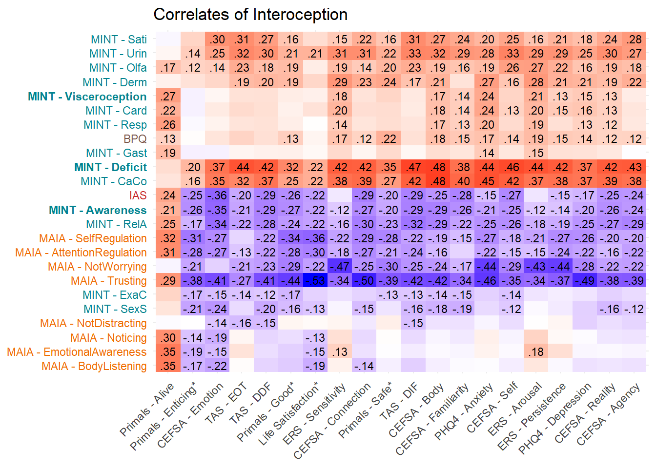
fig2 <- (p_cormint | p_corintero) / p_cor + plot_layout(heights = c(0.4, 0.6))
ggsave("figures/fig2.png", fig2, width=10, height=12, dpi=300)
fig3 <- (mods_moodt$p + theme(axis.text.x = element_blank(), axis.title.x = element_blank()) |
mods_adhd$p + theme(axis.text.x = element_blank(), axis.title.x = element_blank()) |
mods_asd$p + theme(axis.text.x = element_blank(), axis.title.x = element_blank())) /
(mods_central$p | mods_autonomic$p | mods_immune$p) +
plot_layout(guides = "collect") +
plot_annotation(title = "Predictive Performance of Interoceptive Questionnaires",
subtitle = "ROC Curves",
theme = theme(plot.title = element_text(face="bold", hjust = 0.5, size = rel(1.4)),
plot.subtitle = element_text(hjust = 0.5, size = rel(1.25))))
fig3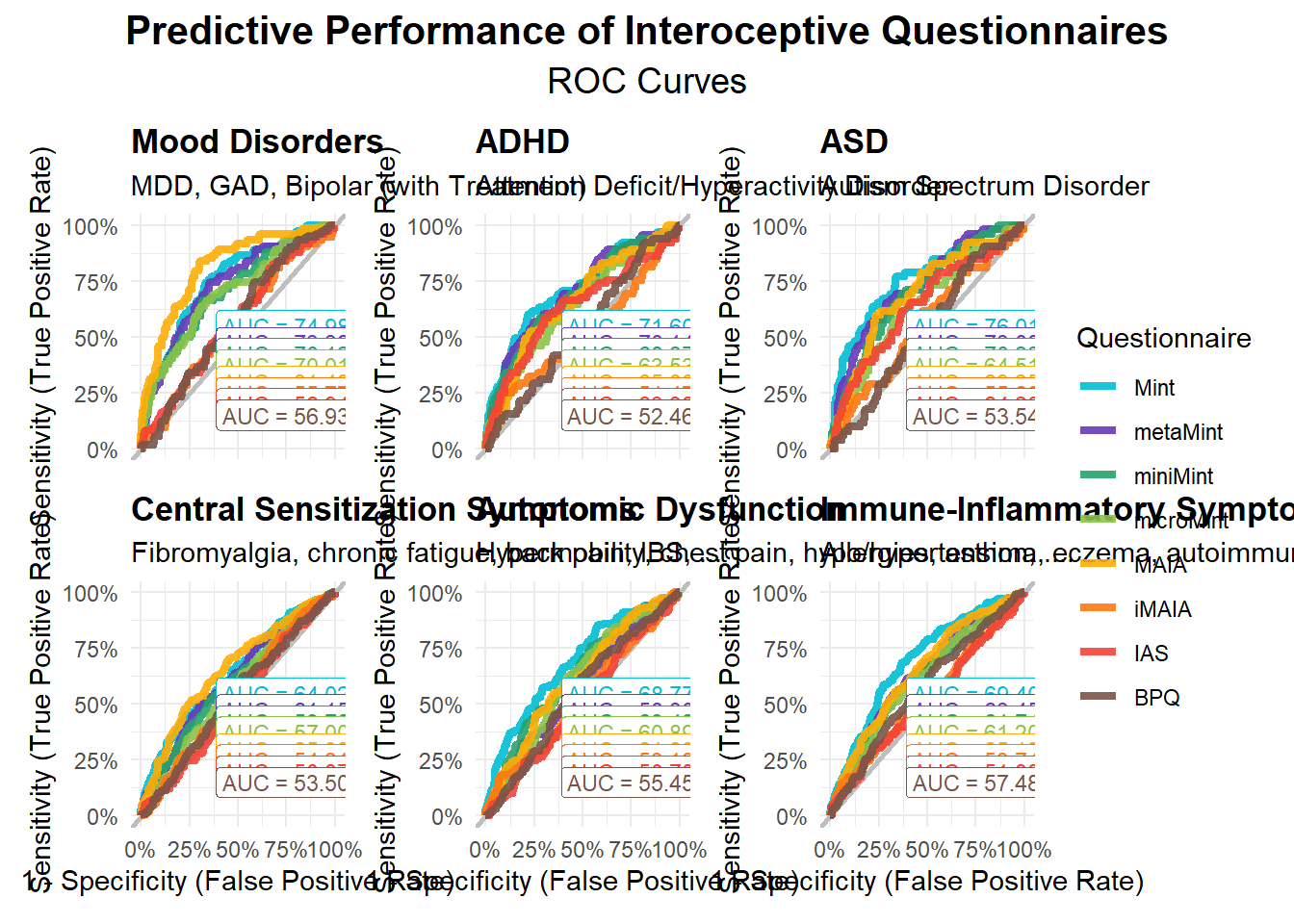
ggsave("figures/fig3.png", fig3, width=13, height=9, dpi=300)