How to extract individual scores from repeated measures
We compare different methods (individual models, Bayesian models with informative priors, random effects from mixed models) to extract individual scores from repeated measures tasks.
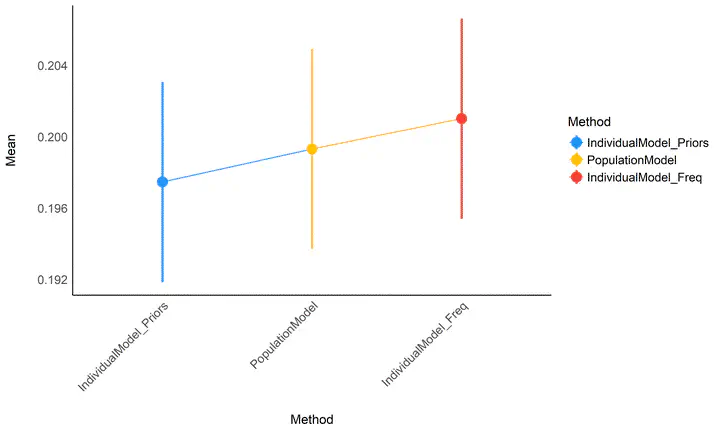 Absolute difference between true individual scores and the scores estimated via different methods.
Introduction
Many psychology fields require to extract individual scores, i.e., point-estimates (i.e., a single value) for a participant/patient, to be used as an index of something and later interpreted or re-used in further statistical analyses. This single index is often derived from several “trials”. For instance, the reaction times in the condition A (let’s say, the baseline) will be averaged together, and the same will be done with the condition B. Finally, the difference between these two means will be used an the individual score for a given participant.
However, we can intuitively feel that we lose a lot of information when averaging these scores. Do we deal appropriately with the variability related to individuals, conditions, or the noise aggravated by potential outliers? This is especially important when working with a limited amount of trials.
With the advent of recent computational advances, new easy-to-implement alternatives emerge. For instance, one can “model” the effects at an individual level (e.g., the simplest case, for the two conditions paradigm described above, would be a linear regression with the condition as a unique predictor), and use the parameters of each model as individual scores (e.g., the “slope” coefficient of the effect of the manipulation), rather than the raw mean. This opens up the possibility of including covariates and take into account other sources of known variability, which could lead to better estimates.
However, individual models are also sensitive to outliers and noise. Thus, another possibility is to model the effects at the population level and, at the same time, at the individual level. This can be achieved by modelling the participants as a random factor in a mixed model. In this case, the individual estimates might benefit from the population estimates. In other words, the effects at the population level will “constrain” or “guide” the estimation at an individual level to potentially limit extreme parameters.
Unfortunately, the above method requires to have all the data at hand, to be able to fit the population model. This is often not the case in on-going acquisition, or in neuropsychological contexts, in which the practitioners simply acquire data for one patient, and have to compute individual scores, without having access to the detailed population data. Thus, an in-between alternative could make use of Bayesian models, in which the population effects (for instance, the mean effect of the condition) could be entered as an informative prior in the individual models to, again, “guide” the estimation at an individual level and hopefully limit the impact of noise or outliers observations.
In this post, the aim is to compare these 4 methods (basic individual model - equivalent to using the raw mean, population model, individual model with informative priors) in recovering the “true” effects using a simulated dataset.
Results
Generate Data
We generate several datasets in which we manipulate the number of participants, in which the score of interest is the effect of a manipulation as compared to a baseline condition. 20 trials per condition will be generated with a known “true” effect (the centre of the distribution from which the data is generated). Gaussian noise of varying standard deviation will be added to create a natural variability (See the functions’ definition below).
library(tidyverse)
library(easystats)

data <- get_data(n_participants=1000, n_trials=20)
results <- get_results(data)
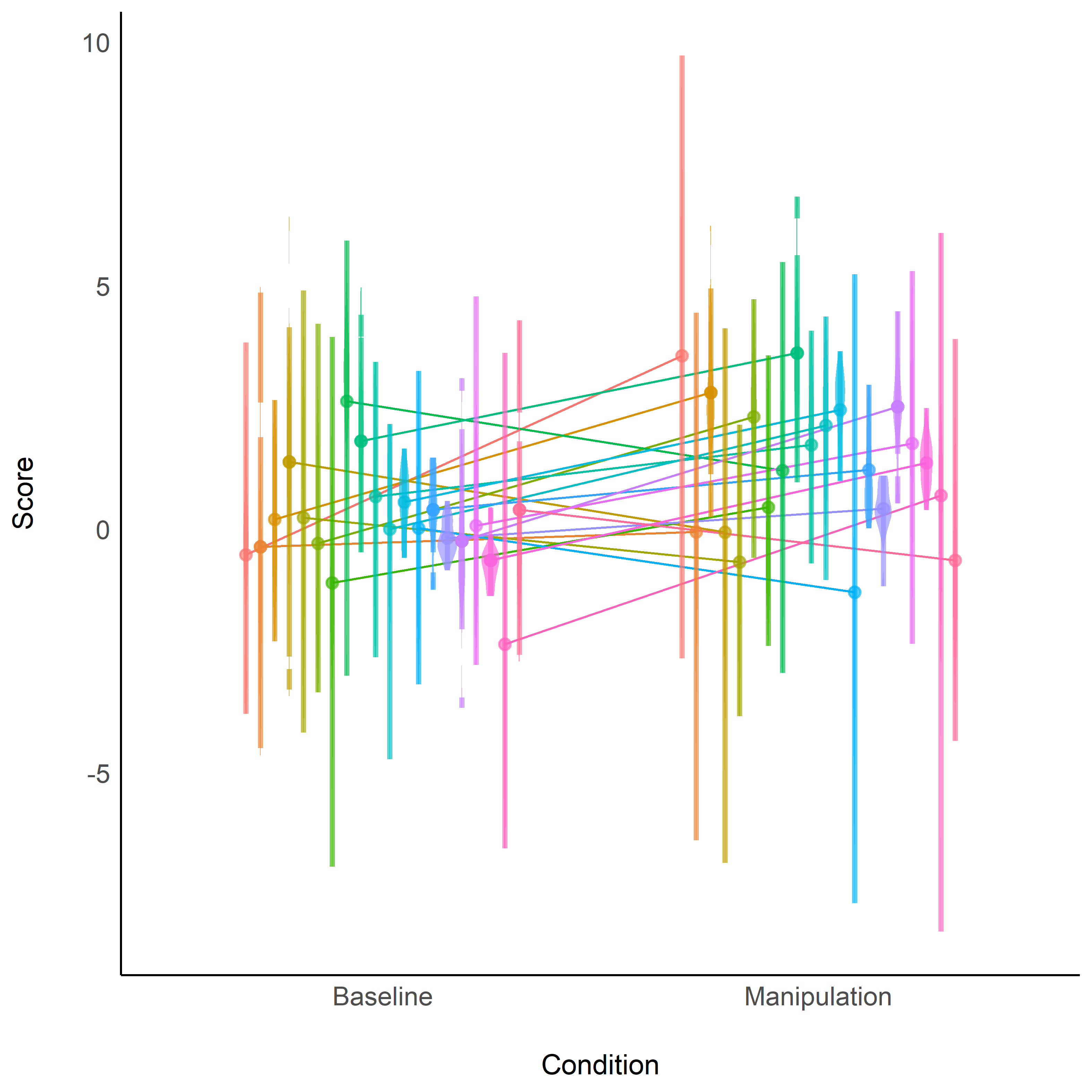
Figure 1: *Example of a dataset containing 20 participants (shown with different colors). As can be seen, we introduced modulations in the inter- and intra- individual variability.*
We will then compare the scores obtained by each method to the “true” score of each participant by substracting them from one another. As such, for each method, we obtain the absolute “distance” from the true score.
Fit model
Contrast analysis will be applied to compare the different methods together.
model <- lm(Diff_Abs ~ Method, data=results)

modelbased::estimate_contrasts(model) %>%
  arrange(Difference) %>%
  mutate(Level1 = stringr::str_remove(Level1, "Diff_"),
         Level2 = stringr::str_remove(Level2, "Diff_")) %>%
  select(Level1, Level2, Difference, CI_low, CI_high, p)
## Level1                 | Level2                 | Difference |            CI |      p
## -------------------------------------------------------------------------------------
## IndividualModel_Priors | PopulationModel        |  -1.85e-03 | [-0.01, 0.01] | > .999
## IndividualModel_Freq   | PopulationModel        |   1.70e-03 | [-0.01, 0.01] | > .999
## IndividualModel_Freq   | IndividualModel_Priors |   3.55e-03 | [-0.01, 0.01] | > .999
Visualize the results
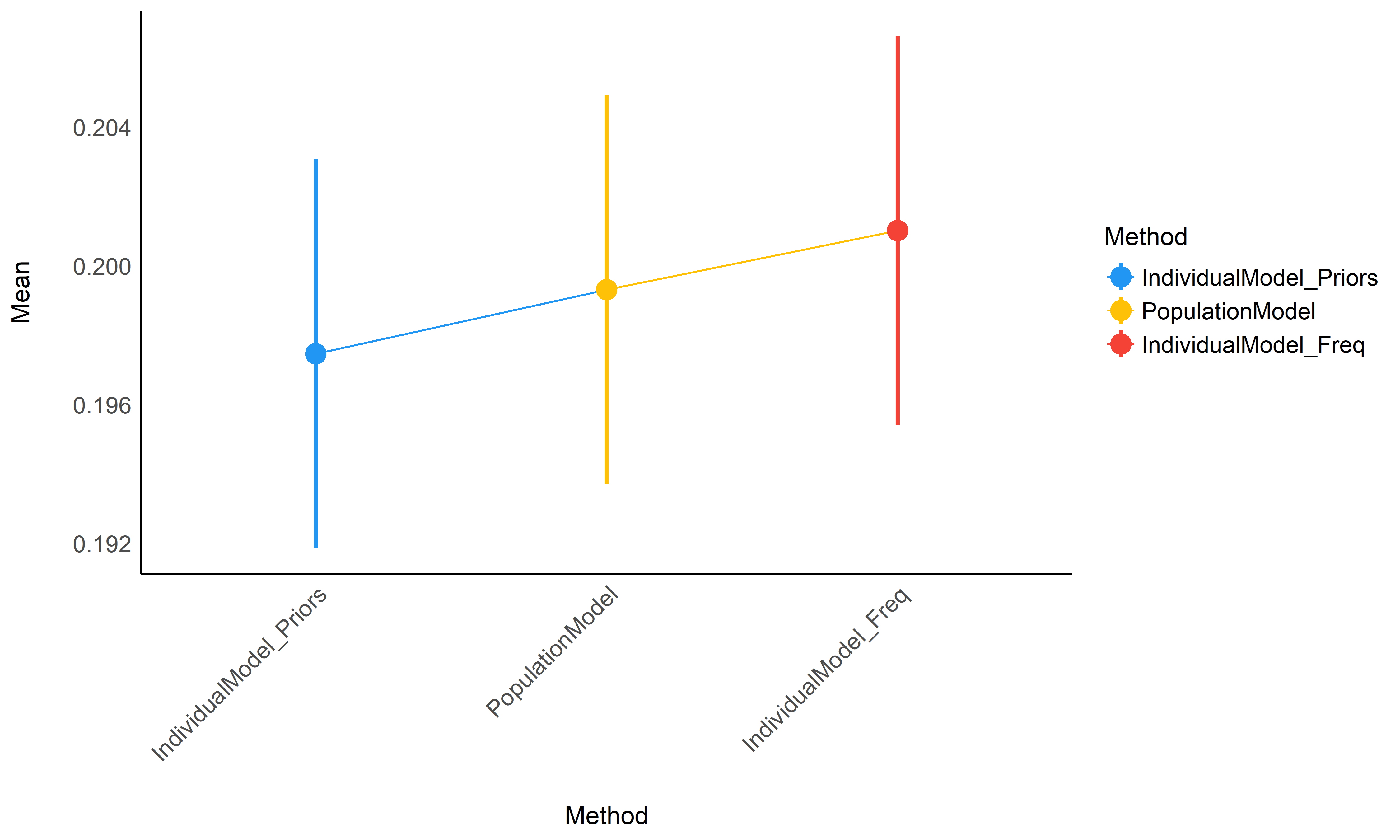
Figure 2: *Average accuracy of the different methods (the closest to 0 the better).*
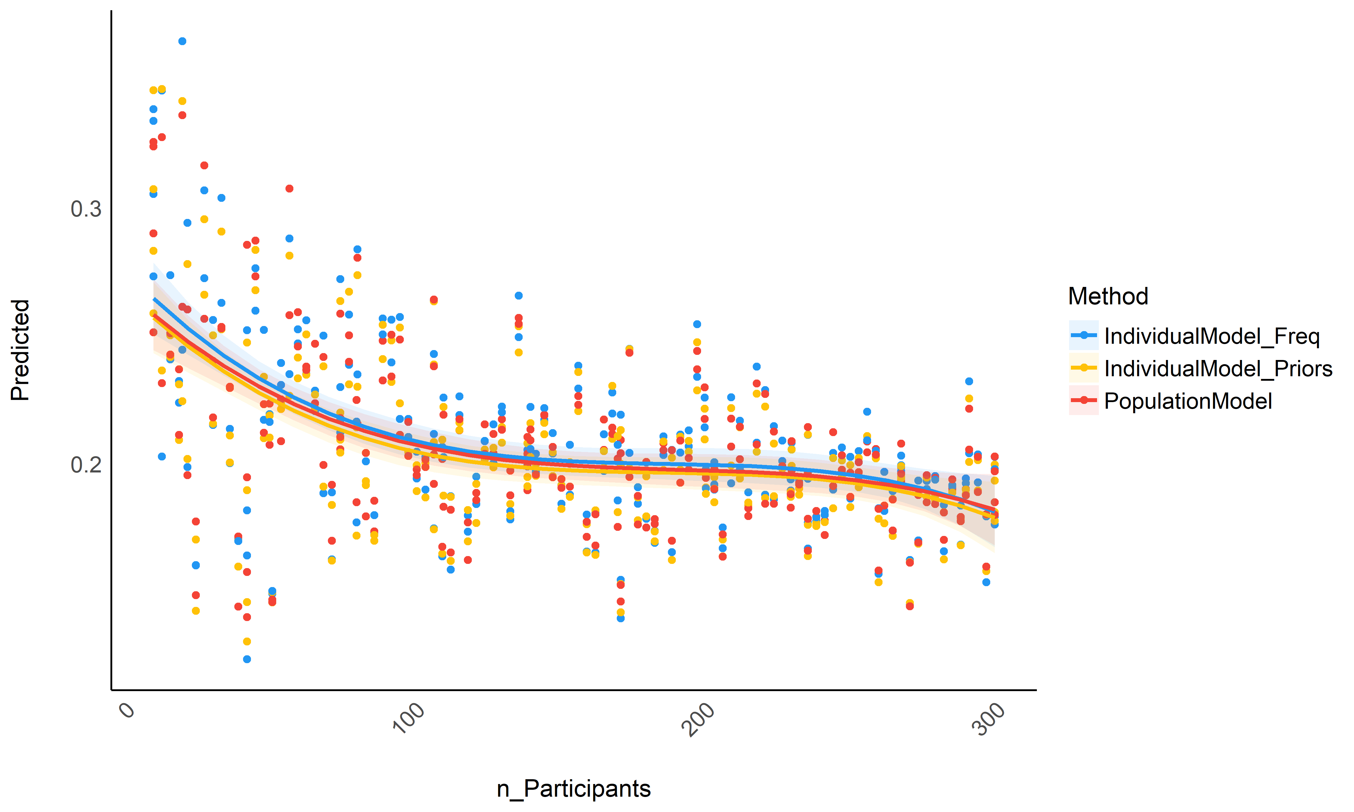
Figure 3: *Accuracy depending on the number of total participants in the dataset.*
Conclusion
Though not significantly different, it seems that raw basic estimates (that rely only on the individual data) perform consistently worse than the population model or individual models informed by priors, especially for small datasets (between 10 and 100 participants) - though again, the difference is tiny in our simulated dataset. In the absence of the whole population dataset, it seems that using individual Bayesian model with informative priors (derived from the population model) is a safe alternative.
Functions
library(tidyverse)
library(easystats)
library(rstanarm)
library(ggdist)


# Get data ----------------------------------------------------------------

get_data <- function(n_participants = 10, n_trials = 20, d = 1.5, var = 3, noise = 0.1) {
  scores_baseline <- rnorm(n_participants, 0, 1)
  scores_condition <- rnorm(n_participants, d, 1)
  variances <- rbeta(n_participants, 2, 8)
  variances <- 0.1 + variances * (var / max(variances)) # Rescale
  noise_sd <- abs(rnorm(n_participants, 0, noise))

  data <- data.frame()
  for (i in 1:n_participants) {
    a <- rnorm(n_trials, scores_baseline[i], variances[i])
    b <- rnorm(n_trials, scores_condition[i], variances[i])
    a <- a + rnorm(n_trials, 0, noise_sd[i]) # Add noise
    b <- b + rnorm(n_trials, 0, noise_sd[i]) # Add noise
    data <- rbind(data, data.frame(
      "Participant" = sprintf("S%02d", i),
      "Y" = c(a, b),
      "Score_True" = rep(c(scores_baseline[i], scores_condition[i]), each = n_trials),
      "Condition" = rep(c("Baseline", "Manipulation"), each = n_trials)
    ))
  }
  data
}


# Visualize data -----------------------------------------------------------

p <- get_data(n_participants = 20) %>%
  group_by(Participant, Condition) %>%
  mutate(mean = mean(Y)) %>%
  ggplot(aes(y = Y, x = Condition, fill = Participant, color = Participant, group = Participant)) +
  geom_line(aes(y = mean), position = position_dodge(width = 0.66)) +
  ggdist::stat_eye(point_interval = ggdist::mean_hdi, alpha = 0.66, position = position_dodge(width = 0.66), .width = c(0.95)) +
  ylab("Score") +
  theme_modern() +
  theme(legend.position = "none")
ggsave("individual.png", p, width = 7, height = 7, dpi = 450)


# Get results -------------------------------------------------------------


get_results <- function(data) {

  # Raw method ----

  results <- data %>%
    group_by(Participant, Condition) %>%
    summarise_all(mean) %>%
    rename("Score_Raw" = "Y") %>%
    arrange(Condition, Participant) %>%
    ungroup()


  # Population model ----

  model <- lme4::lmer(Y ~ Condition + (1 + Condition | Participant), data = data)

  fixed <- insight::get_parameters(model, effects = "fixed")$Estimate
  random <- insight::get_parameters(model, effects = "random")$Participant

  # Transform coefs into scores
  pop_baseline <- random[, 1] + fixed[1]
  pop_manipulation <- pop_baseline + random[, 2] + fixed[2]

  results$Score_PopulationModel <- c(pop_baseline, pop_manipulation)


  # Individual model ----

  individual_model_data <- data.frame()
  for (participant in unique(data$Participant)) {
    cat(".") # Print progress

    dat <- data[data$Participant == participant, ]

    # Frequentist
    model1 <- lm(Y ~ Condition, data = dat)
    nopriors <- parameters::parameters(model1)$Coefficient

    # Bayesian without priors
    # model2 <- stan_glm(Y ~ Condition, data = dat, refresh = 0)
    # bayes <- parameters::parameters(model2)$Median

    # Bayesian with Priors
    model3 <- stan_glm(Y ~ Condition,
      data = dat,
      refresh = 0,
      prior = normal(fixed[1]),
      prior_intercept = normal(fixed[2])
    )
    priors <- parameters::parameters(model3)$Median

    individual_model_data <- rbind(
      individual_model_data,
      data.frame(
        "Participant" = c(participant, participant),
        "Condition" = c("Baseline", "Manipulation"),
        "Score_IndividualModel" = c(nopriors[1], nopriors[1] + nopriors[2]),
        # "Score_IndividualModel_Bayes" = c(bayes[1], bayes[1] + bayes[2]),
        "Score_IndividualModel_Priors" = c(priors[1], priors[1] + priors[2])
      )
    )
  }

  results <- merge(results, individual_model_data)


  # Clean output ----

  diff <- results %>%
    mutate(
      # Diff_Raw = Score_True - Score_Raw,
      Diff_PopulationModel = Score_True - Score_PopulationModel,
      Diff_IndividualModel = Score_True - Score_IndividualModel,
      # Diff_IndividualModel_Bayes = Score_True - Score_IndividualModel_Bayes,
      Diff_IndividualModel_Priors = Score_True - Score_IndividualModel_Priors
    ) %>%
    select(Participant, Condition, starts_with("Diff")) %>%
    pivot_longer(starts_with("Diff"), names_to = "Method", values_to = "Diff") %>%
    mutate(Diff_Abs = abs(Diff))

  diff
}


# Analysis ----------------------------------------------------------------
results <- data.frame()
for(n in seq.int(10, 300, length.out = 10)){
  data <- get_data(n_participants = round(n), n_trials = 20)
  rez <- get_results(data) %>%
    select(-Participant) %>%
    group_by(Condition, Method) %>%
    summarise_all(mean) %>%
    mutate(n_Participants = n,
           Method = as.factor(Method),
           Dataset=paste0("Dataset", round(n, 2)))
  results <- rbind(results, rez)

  print(n) # Print progress
}

# model <- mgcv::gam(Diff_Abs ~ Method + s(n_Participants, by = Method), data = results)
model <- lm(Diff_Abs ~ Method * poly(n_Participants, 3), data = results)

parameters::parameters(model)


contrasts <- modelbased::estimate_contrasts(model) %>%
  arrange(Difference) %>%
  mutate(
    Level1 = stringr::str_remove(Level1, "Diff_"),
    Level2 = stringr::str_remove(Level2, "Diff_")
  ) %>%
  select(Level1, Level2, Difference, CI_low, CI_high, p)


# Visualize results ---------------------------------------------------------
p <- modelbased::estimate_means(model) %>%
  arrange(Mean) %>%
  mutate(
    Method = stringr::str_remove(Method, "Diff_"),
    Method = factor(Method, levels = Method)
  )  %>%
  ggplot(aes(x = Method, y = Mean, color = Method)) +
  geom_line(aes(group = 1)) +
  geom_pointrange(aes(ymin = CI_low, ymax = CI_high), size = 1) +
  theme_modern() +
  theme(axis.text.x = element_text(angle = 45, hjust = 1)) +
  scale_color_material()
ggsave("featured.png", p, width = 10, height = 6, dpi = 450)


p <- modelbased::estimate_relation(model) %>%
  mutate(Method = stringr::str_remove(Method, "Diff_"))  %>%
  ggplot(aes(x = n_Participants, y = Predicted)) +
  geom_point(data=mutate(results, Method = stringr::str_remove(Method, "Diff_")),
             aes(y=Diff_Abs, color = Method)) +
  geom_ribbon(aes(ymin=CI_low, ymax=CI_high, fill=Method), alpha=0.1) +
  geom_line(aes(color = Method), size=1) +
  theme_modern() +
  theme(axis.text.x = element_text(angle = 45, hjust = 1)) +
  scale_color_material() +
  scale_fill_material()
ggsave("n_participants.png", p, width = 10, height = 6, dpi = 450)


# Save results ------------------------------------------------------------


d <- list("results" = results, "model" = model, "contrasts" = contrasts)
save(d, file = "data.Rdata")
References
You can reference this post as follows:
- Makowski, D. (2020, September 14). How to extract individual scores from repeated measures. Retrieved from https://dominiquemakowski.github.io/post/individual_scores/
Thanks for reading! Do not hesitate to share this post, and leave a comment below 🤗
🐦 And don’t forget to join me on X @Dom_Makowski
Dominique Makowski
Lecturer in Psychology
Trained as neuropsychologist and CBT psychotherapist, I am currently working as a lecturer at the University of Sussex, on the neuroscience of reality perception.